
Cosmic Rays in the Atmosphere
 *Source is C. R. Nave, Cosmic Rays, HyperPhysics.*
Cosmic Rays in the Atmosphere
Muons and neutrinos
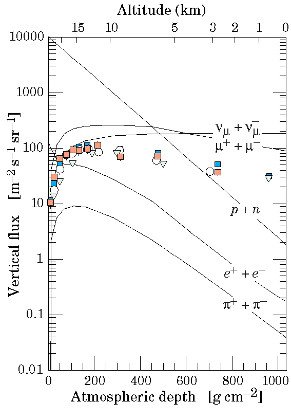
- Muons and neutrinos are produced in decays of mesons which are themselves produced by interactions of CR particles with air nuclei.
- They are the dominant flux at sea level and the only ones that can penetrate deep underground.
- Electrons and nucleons fluxes above 1 GeV/$c$ are about 0.2 and 2 m$^{-2}$ s$^{-1}$ sr$^{-1}$ at sea level. Nucleons are the degraded remnants of the primary cosmic radiation. At sea level about 1/3 are neutrons.
Cosmic Rays in the Atmosphere
Muons and neutrinos productions
The most important channels for muon and neutrino production are:
Two body decays $$\pi^{\pm} \rightarrow \mu^{\pm} + \nu_{\mu}({ \bar \nu_\mu}) \rm{\;\; (\sim 100\%)}$$ $$K^{\pm} \rightarrow \mu^{\pm} + \nu_{\mu}({\bar \nu_\mu}) \rm{\;\; (\sim 63.5\%)}$$
Three body decay $$K_L \rightarrow \pi^{\pm} e^{\pm}\nu_e({\bar \nu_e}) \rm{\;\; (\sim 38.7\%)}$$
At lower energies, the muon decay is also important:
$$ \mu^{\pm} \rightarrow e^{\pm} + \nu_{e}({\bar \nu_e}) + {\bar \nu_{\mu}}(\nu_\mu)$$The neutrino flavor ratio is: $$\boldsymbol{ \nu_\mu : \nu_e = 2:1}$$
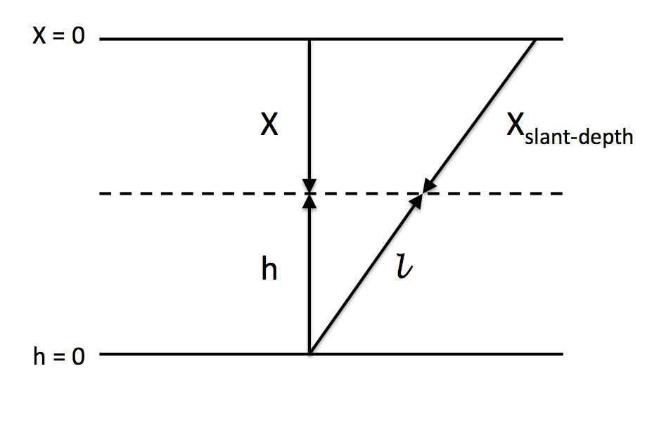
It is important to know the atmosphere to understand the cosmic rays interaction in it. The vertical atmospheric depth, $X$ measured in g/cm$^{2}$ is defined as the integral in altitude of the atmospheric density $\rho$ above the observation level $h$:
$$X =\int_h^{\infty} \rho(h^\prime){\rm d}h^\prime$$The Atmosphere
The isothermal model
In an isothermal atmosphere, the pressure decreases exponentially with increasing height. Since the temperature is assumed to be constant it follows that $\rho$ also changes exponentially and the afore equation can be written as:
$$X = X_0 {\rm e}^{-h/h_0}$$where $X_0$ is 1030 g/cm$^{2}$ is the atmospheric depth at sea level, h = 0, and $h_0$ is the scale height or the height needed to drop presure or density a factor $1/e$.
The Atmosphere
The scale height
The scale height is given by:
$$ h_0 = \frac{R T}{M g_0} $$where $R$ is the ideal gas constant, $T$ is temperature, $M$ is average molecular weight, and $g_0$ is the gravitational acceleration at the planet's surface. Using typical values ($T = 273$ K and $M = 29$ g/mol) we get that $h_0 \sim 8$ km which coincidentally is the approximate height of Mt. Everest.
In reality the temperature changes and hence the scale height decreases with increasing altitude until the tropopause.
This equations are valid for vertical particles, for zenith angles < 60$^\circ$ (for which we can ignore the Earth's curvature) the formula is scaled with $1/\cos{\theta}$ giving the slant depth
The Atmosphere
Mean free paths for Nucleons
The nucleon mean free path, $\lambda_N$, in the atmosphere is given (in g/cm$^2$) by:
$$\lambda_N = \frac{Am_p}{\sigma_N^{air}}$$where $\sigma_N^{air}$ is the nucleon cross-section in air, $A$ is mean the mass number of air nuclei (mainly nitrogen, oxygen) and $m_p$ is the proton mass. Assuming $A \sim 14.5$ and $\sigma_N^{air} \approx$ 300 mb, it corresponds to $\lambda_N \approx 80$g/cm$^{2}$, which corresponds to 11 interaction lengths in $X_0$.
The standard mean free path is: $l = (n\sigma^{air}_N)^{-1}$ where $n$ is the number density of air nuclei ie:
$$n = \frac{N_T}{V}$$Where $N_T$ is the total number of air nuclei and V is total air volume. $\sigma^{air}_N$ is the nucleon-air cross section.
The density mean free path is $\lambda = \rho l$, but $\rho = M_T/V$ and $M_T = N_T * m_air$ where $m_air$ is mass of an air nuclei. Putting everything together:
$$\lambda = \rho l = \frac{N_T m_{air}}{V}\frac{V}{N_T\sigma_{air}} = \frac{m_{air}}{\sigma_{air}}$$where we can use $m_{air} = A m_p$.
The Atmosphere
Mean free path for mesons, $\pi$, K
- The decay mean free path of pions is given by $\lambda =\gamma c \tau_\pi$ where $\gamma$ is the lorentz boost. In units of slant depth is defined as:
where $E$, $m_\pi$, $\tau_\pi$ are the pion energy, mass and lifetime and we defined:
$$\epsilon_\pi = \frac{c\tau_\pi}{m_\pi c^2 h_0}$$as a critial energy when the decay length equals the slant depth.
- The interaction mean free path is the same as nucleon $\lambda_\pi = A m_\pi/\sigma_\pi^{air}$
To go from the decay mean free path to normal units to the mean free path in units of slant depth we used:
$$\begin{align*} \Phi &= \Phi_0 e^{-\lambda l}\\ \frac{d\Phi}{d l} &= -\Phi \frac{1}{\gamma c \tau}\\ dl &= - dh/\cos\theta\\ dX &= -1/h_0 X_0 e^{-h/h_0} dh \end{align*}$$so:
$$ d\Phi = - \Phi \frac{1}{\gamma c \tau \cos\theta} dh = - \Phi \frac{h_0}{X\gamma c\tau \cos\theta} dX = \frac{m c^2 h_0}{E c \tau X \cos \theta} d X$$where we used the fact that $\gamma = \frac{E}{mc^2}$
The Atmosphere
Critical energy for mesons, $\pi$, K
Decay or interaction dominates depending on whether $1/d_\pi$ or $1/\lambda_\pi$ is larger. This in turns depends on the ratio between E and $\epsilon_\pi$. For pions we have:
$$\epsilon_\pi = \frac{c\tau_\pi}{m_\pi c^2 h_0} \approx 115 \;{\rm GeV}$$So we can distinguis two regimes.
For $E \gg \epsilon_\pi$ decay length is much larger than the slant depth, so interaction dominates.
For $E \ll \epsilon_\pi$ decay dominates.
The same formulas can be derived for Kaons.
Muon Fluxes
Energy regimes
Three different regimes are distinguishable:
$E_\mu \leq \epsilon_\mu$, where $\epsilon_\mu \sim 1 {\rm\;GeV}$. In this case muon decay and muon energy loss are important. The muon flux is suppressed.
$\epsilon_\mu \leq E_\mu \leq \epsilon_{\pi,K}$, where $\epsilon_\pi = 115 {\;\rm GeV}$ and $\epsilon_K = 850 {\;\rm GeV}$. In this range all messons decay and muons follow the same spectrum as mesons and hence of CRs. The muon is almost independent of the zenith angle.
$E_\mu \gg \epsilon_{\pi,K}$, Mesons do not decay and muon flux gets suppressed.
Muon Fluxes
Analytical approximation
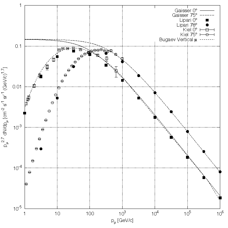
- An approximate extrapolation formula valid when muon decay is negligible ($E_\mu > 100/\cos\theta$ GeV) and the curvature of the Earth can be neglected ($\theta < 70^{\circ}$) is given by the Gaisser parametrization:
where $F_\pi$ and $F_K$ represent the contributions from pions and kaons, respectively: $$ \begin{align*} F\pi(E\mu, \theta) = \frac{1}{1+\frac{1.1 E_\mu \cos\theta}{115 {\;\rm GeV}}} \end{align} $$ $$F_K(E_\mu, \theta) = \frac{0.054}{1+\frac{1.1 E_\mu \cos\theta}{850{\;\rm GeV}}} $$
%matplotlib inline
import matplotlib.pyplot as plt
import numpy as np

def muons(cangle, E):
    a = 1./(1.+ 1.1*E*cangle/115.)
    b = 0.054/(1.+ 1.1*E*cangle/850.)
    return 0.14 *E**-2.7 *(a + b)
import seaborn as sea
#sea.set_style("whitegrid")
sea.set_context("poster")
fig = plt.figure(figsize=(6,8))
ax = plt.subplot(111)
ax.set_xscale("log")
ax.set_yscale("log")
ax.set_ylim(1e-4, 3e-1)
ax.set_ylabel("$E_\mu^{2.7} dN_\mu/dE_\mu [cm^{-2}s^{-1} (GeV)^{1.7}]$", fontsize=20)
ax.set_xlabel("$E_\mu(GeV)$", fontsize=20)

E = np.arange(1e0, 1e6, 10)

ax.plot(E, E**2.7*muons(np.cos(60*np.pi/180.),E), label=r"$\theta = 60^{\circ}$")
ax.plot(E, E**2.7*muons(np.cos(0*np.pi/180.),E), label=r"$\theta = 0^{\circ}$")
plt.legend()
plt.show()

Muon Fluxes
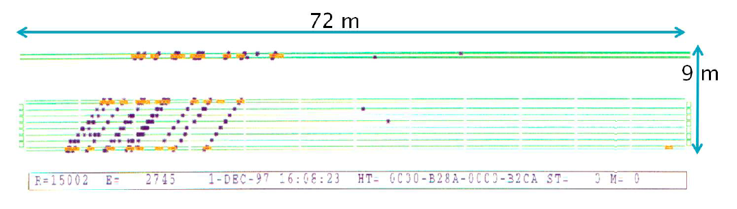
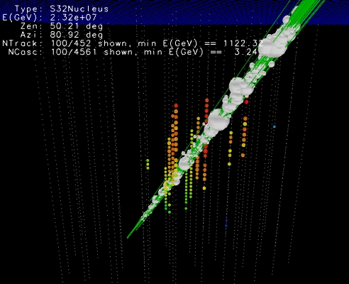
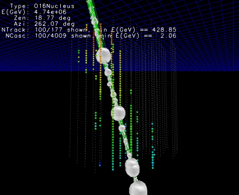
Bundles
Sometimes muons also come in groups or bundles of parallel muons originated from the same primary CR. Muon bundles sometime look like a single high energy muon. The multiplicity (number of muons in the bundle) if can be measured is correlated with the mass of the orignal CR.
Muons
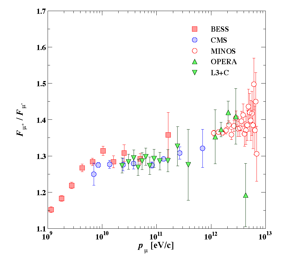
Charge Ratio
Neutrinos
Fluxes
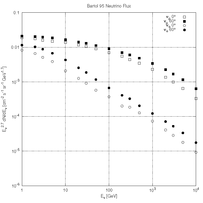
- Neutrinos are the most abundant CR product at sea level, yet they have only recently (compared to other particles) measured due to their extremely low cross-section.
- The process giving neutrino fluxes are the same as for the muons (we saw already) plus the muon decay. Taking into account the decay of pions, kaons and muons gives to a flavor ratio of: $\nu_\mu : \nu_e = 2:1$ and $\nu_e/{\bar \nu_e} \sim \mu^+/\mu^-$
- At few GeV (> $\epsilon_\mu$) muons will not decay and $\nu_e$ will be supressed as the main source of $\nu_e$ is the muon decay.
Neutrinos
Fluxes and kinematics
As mentioned neutrinos and muons are strongly correlated. However due the two-body kinematics, the energy spectra of the $\nu$’s and $\mu$’s from mesons decay are different. For example, the energy of the muon in CM is given by:
$$E_\mu^{cm} = (m_\pi^2 + m_\mu^2)/2m_\pi = 109.8 {\rm\; MeV}$$and for the neutrino:
$$E_\nu^{cm} = (m_\pi^2 - m_\mu^2)/2m_\pi = 29.8 {\rm \; MeV}$$In the laboratory system, the energies are boosted by the Lorentz factor $\gamma= E_\pi /m_\pi$, but as can be seen muon carry a much larger fraction of energy than neutrinos. For energies about 1 TeV $ < E_\nu < 10^3$ TeV, the angle averaged atmospheric $\nu_\mu + {\bar \nu_\mu}$ can be approximated by a power law spectrum:
$$\frac{{\rm d}N_{\nu_\mu + {\bar \nu_\mu}}}{{\rm d}E_\nu} = 7.8 \times 10^{-11}\left(\frac{E_\nu}{1{\rm\;TeV}}\right)^{-3.6} {\rm \; cm^2\;s^{-1}\;sr^{-1}\;GeV^{-1}}$$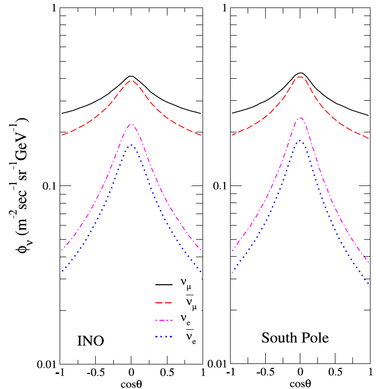 Calculated neutrino flux at 1,300 m depth with $E_\nu = 10$ GeV. Taken from [arXiv:1210.5154](http://arxiv.org/abs/1210.5154)
 The peak at the horizon in the atmospheric neutrino flux is due to the so-called secant theta effect. This effect occurs because pions and kaons that are produced nearly skimming the Earth have more flight time in less dense atmosphere, so they have more chance to decay than interact.
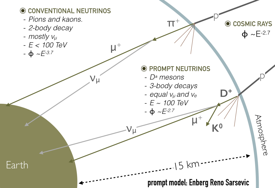
Prompt Fluxes
Apart from kaons and pions, charmed messons will also be produced in the atmosphere. Charm particles have lifetimes so short they almost alway decay before interacting. Muons and neutrinos from charm decay are called prompt muons/neutrinos. There are two peculiarities of the prompt fluxes:
- The energy spectrum follows the one of the primary cosmic rays.
- Since there is no competition between decay and interaction of the charm particle, the prompt flux is isotropic.
- They produced the same amount of $\nu_\mu$ and $\nu_e$.
Prompt fluxes have not been observed yet.
Summary of neutrino atmospheric fluxes
Muon Interactions

- Ionisation.The continuous energy loss of muons passing through a medium as it ionize the material along the path. Diagram a).
- Bremsstrahlung. In the electric field of a nucleus or atomic electrons, muons can radiate high energy photons as shown in diagram b)
- Pair production. A muon can radiate a virtual photon which, again in the electric field of a nucleus, can convert into a real $e^+e^-$ pair. Diagram c)
- Photonuclear interactions. A muon can radiate a virtual photon which directly interacts with a nucleus in the muon propagation medium. The interaction is either electromagnetic or following the fluctuation of the photon into a quark-antiquark pair (i.e. a virtual vector meson). Diagram d)
Muon Interactions
Muon Energy losses
The energy losses due to ionization are continuous while in radiation processes the energy is lost in bursts along the muon path. The energy loss for muons at high energy can be simplified to:
$$\frac{{\rm d}E_\mu}{{\rm d}X} = -\alpha -\beta E_\mu$$where $X$ is the thickness of the material (in g/cm$^2$), $\alpha$ is the energy loss due to ionization and $\beta = \beta_{br} + \beta_{pair} + \beta_{ph}$ are the three discrete energy loss processes: bremsstrahlung, electron-positron production and electromagnetic interaction with the nuclei. Thickness is also given sometimes in units of meters water equivalent (1 m.w.e. = 10$^2$ g/cm$^2$).
The critical energy is when both losses are equal, ie $\epsilon_\mu = \alpha/\beta$. Typical values are $\alpha \simeq 2$ MeV g$^{-1}$cm$^2$ and $\beta \simeq 4 \times 10^{-6}$g$^{-1}$cm$^2$, so $\epsilon_\mu \approx 500$ GeV.
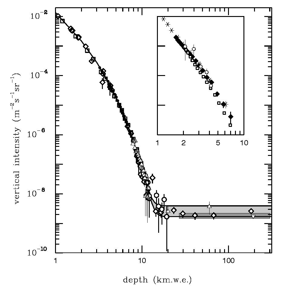
Muon Range
$$ R(E_\mu) = \frac{1}{\beta}{\rm In}\left( 1 + \frac{E_\mu}{\epsilon_\mu}\right)$$
Assuming the muon spectrum at sea level can be approximated to a power law $I_\mu(>E_\mu) = AE_\mu^{-\gamma}$ and using the relationship between range and energy we can write the *depth-intensity relation* (DIR):
$$I_\mu(>E_\mu, R) = A\left[\frac{\alpha}{\beta}(e^{\beta R} - 1)\right]^{-\gamma}$$
Neutrino Interactions
Weak interaction
- Neutrinos feel only the weak force thus interactions with matter mediated by W and Z bosons with cross-sections typical of weak processes.
Feynman diagrams factor along two lines:
- Neutral current (NC) interactions - exchange of Z
Charged current (CC) interaction - exchange of W$^{\pm}$
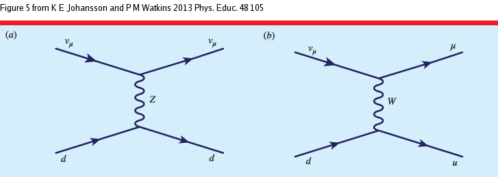
Neutrinos will scatter from electrons as well as nuclear matter.
Below 1 GeV neutrinos interact with hadronds via elastic or quasielastic scattering.
At $E_\nu \gg$ 1 GeV neutrinos do not scatter on hadronds as a compound of quarks, they start to see the quarks, Deep Inelastic Scattering.
Neutrinos Interactions
Neutrino cross-sections at GeV energies
- The anti-neutrino cross-section at GeV energies is a factor ~2 lower than the neutrino cross-section due to the helicity.
At $E_\nu \gg 1$ GeV the DIS cross-section can be approximated to:
$$\sigma_{\nu p} \simeq 0.69 \times 10^{-38} \left(\frac{E_\nu}{ 1 {\rm\; GeV}}\right) {\rm \; cm}^2$$$$\sigma_{{\bar\nu} p} \simeq 0.35 \times 10^{-38}\left(\frac{E_\nu}{ 1 {\rm\; GeV}}\right){\rm \; cm}^2$$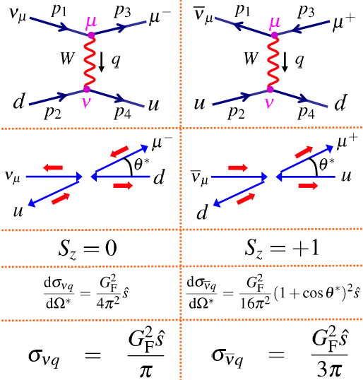
Earth is transparent to GeV neutrinos
from astropy import constants as ct
from astropy import units as u
#Earth mass
print ct.M_earth

#Neutron/proton mass
print ct.m_p

#Earth radius
print ct.R_earth

#number of nucleons
N = ct.M_earth/ct.m_n

#Earth volume
Ve = 4/3*np.pi*ct.R_earth**3

#Nucleon density
Nd = N/Ve


#Cross section
s = 1e-38 * u.cm**2
#Mean free path:
L = 1/(s * Nd.to(1/u.cm**3))

print "The mean free path is: ", L.to(u.km)
Neutrinos Interactions
Neutrino cross-sections at TeV energies
At low energies the valence quark parton distribution dominates and both the neutrino NC and CC cross-section grows linear with energy since the transfer momemtum $q^2 \ll M_{W,Z}$ and so the propagator term is $\sim 1/M^2_{W,Z}$
Above 10$^{4}$ GeV where the gauge-boson propagator restricts the momentum transfer to values near $M_{W,Z}$ ($\sim 1/(q^2 - M^2_{W,Z})$) and damps the cross-section increase.
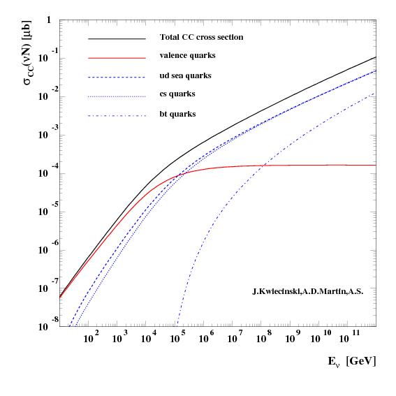 Calculated neutrino cross sections taken from astro-ph/0310636
Neutrino Interactions
High energy Cross-Sections
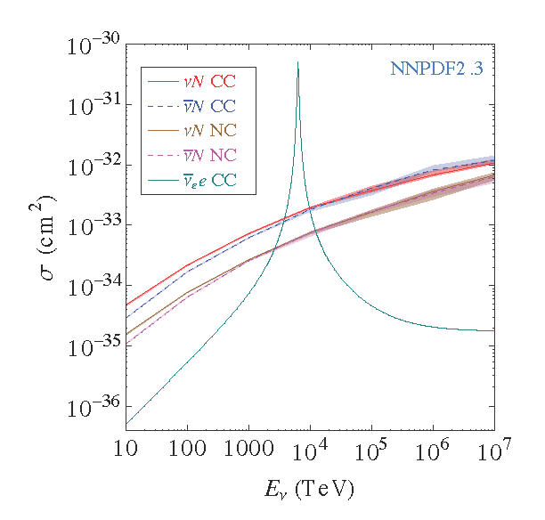 Calculated neutrino cross sections taken from [arXiv:1309.1764](http://arxiv.org/abs/1309.1764)
At high energies the asymetry between neutrinos and antineutrinos is lost due to the interaction with sea quarks ($q\bar{q}$)
Neutrinos interact mostly with hadrons (quarks) instead of electrons due the their larger target mass. However at $E_\nu \approx 6.3$ PeV the Glashow resonance appears: ${\hbar \nu_e} + e \rightarrow W$ making the cross-section higher than the one with hadrons.
Earth Opaque to PeV Neutrinos
At about 100 TeV the mean free path for neutrino-nucleus scattering is about 10$^{10}$ c.m.w.e. which is about the matter thickness along the Earth diameter.
This means that UHE neutrino observatories (like IceCube) the flux of neutrinos comming from the nadir is stronly suppressed.
There is only one exception. A very high energy beam of $\nu_\tau$ at one side of the Earth $E\gg 1$ PeV can end up at the other side as lower energy $\nu_\tau, \nu_e,\nu_\mu$ thought the tau regeneration effect: $\nu_\tau \rightarrow \tau \rightarrow \nu_\tau$
Neutrino signatures in a detector
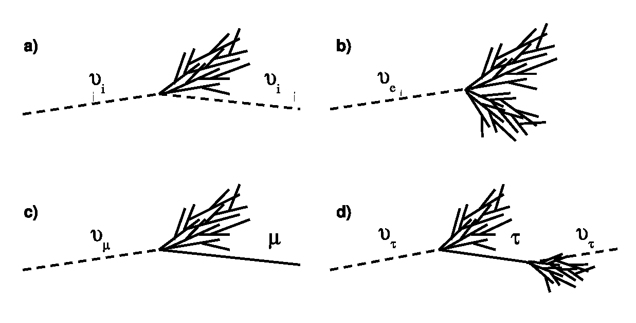
- b) In CC $\nu_e$ interactions an hadronic and EM shower initiated by the $e$ is produced. About 20% of the energy goes inthe hadronic shower and 80% to the lepton and therfore to the EM shower.
- d) In CC $\nu_\tau$ d) interaction again an hadronic and EM shower are produced as the $\tau$ decays almost inmediately to pions or other charge leptons. In the decay another $\nu_\tau$ is produced tau regeneration effect. At very high energyes the two showers can be separated giving a double bang signature or a lollipop if the first shower happens outside the detector.
- c) In CC $\nu_\mu$ the muon only undergoes radiation losses (not ionization) and hence the track of the muon can be reconstructed.
- a) In NC only an hadronic shower is visible.
Event rate in an underground experiment.
An estimate of the detection rate of neutrino events is equivalent to calculate the rate of a neutrino-induced muon/cascades flux:
$$R(E_{vis}, \theta) = \int_{E_{vis}} P_{\nu\rightarrow l} (E_\nu, E_{vis}) P_{shadow}(\theta, E_\nu) \frac{{\rm d}N_\nu}{{\rm d}E_\nu}{\rm d}E_\nu$$where
- $P_{\nu\rightarrow l}(E_\nu, E_{vis})$. Probability that a neutrino interacts with an nucleus to produce a $\mu$ or an EM or hadronic cascade with a minimum energy $E_{vis}$ visible in the detector.
- $P_{shadow} (\theta, E_\nu)$. Probability of neutrino with zenith angle $\theta$ and energy $E_\nu$ of being absorved by Earth.
- ${{\rm d}N_\nu}/{{\rm d}E_\nu}$. Neutrino flux at the surface.
Interaction probability: $P_{\nu\rightarrow l}$
The probability of a neutrino to produce a letpon or shower visible in the detector can be writen as:
$$P_{\nu \rightarrow l} = N_A \int_{E_{min}}^{E_\nu} {\rm d}E_l \frac{{\rm d}\sigma}{{\rm d}E_l}r_l(E_l, E_{vis})$$where $r_l$ is the detection range of the produced lepton/cascade with energy $E_l$ ending with the minimal energy $E_{vis}$, and ${{\rm d}\sigma}/{{\rm d}E_l}$ is the neutrino cross-section to produce a lepton/cascade with energy $E_l$.
At high energy the event rate is dominated by neutrino-induced muons due to the long range of the high energy muons.
Earth Shadow: $P_{shadow}$
The mean free path of neutrinos can be expressed as $\lambda = (N_A \sigma_{tot})^{-1}$. The shadow fact then can be expressed as:
$$P_{shadow} = e^{-N_A \sigma_{tot} X(\theta)}$$Where $X(\theta)$ is the column depth travelled by the neutrino through the Earth with a zenith angle $\theta$.
See Exercises 2 for an evaluation of the event rate in an underground detector.
Oscillations
Neutrino Oscillations
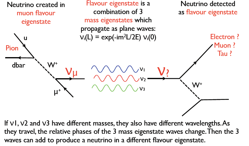
As a result of these changes in relative phases, neutrinos oscillate from one flavor to another as they travel. Low-energy neutrinos oscillate in a shorter distance than high-energy neutrinos.
A curious aspect of quantum physics is that only the probability of the flavor of neutrino changes as it travels.
The neutrino only becomes a definite flavor when it interacts in a detector - by finding whether an electron, muon, tau is created.
The PMNS Matrix
The Pontecorvo-Maki-Nakagawa-Sakata matrix is the one that relates the mass eingenstates with the flavor eingenstates:
$$\begin{pmatrix} \nu_e \\ \nu_\mu \\ \nu_\tau \end{pmatrix} = U_{PMNS} \begin{pmatrix} \nu_1 \\ \nu_2 \\ \nu_1 \end{pmatrix}$$with:
$$ \begin{align*} U_{PMNS} &= \begin{pmatrix} c_{12}c_{13} & s_{12}c_{13} & s_{13}e^{-i\delta} \\ -s_{12}c_{23} - c_{12}s_{23}s_{13}e^{i\delta} & c_{12}c_{23} - s_{12}s_{23}s_{13}e^{i\delta} & s_{23}c_{13} \\ s_{12}s_{23} - c_{12}c_{23}s_{13}e^{i\delta} & -c_{12}s_{23} - s_{12}c_{23}s_{13}e^{i\delta} & c_{23}c_{13} \end{pmatrix} \\ &= \begin{pmatrix} 1 & 0 & 0 \\ 0 & c_{23} & s_{23} \\ 0 & -s_{23} & c_{23} \end{pmatrix} \begin{pmatrix} c_{13} & 0 & s_{13}e^{-i\delta} \\ 0 & 1 & 0 \\ -s_{13}e^{i\delta} & 0 & c_{13} \end{pmatrix} \begin{pmatrix} c_{12} & s_{12} & 0 \\ -s_{12} & c_{12} & 0 \\ 0 & 0 & 1 \end{pmatrix} \end{align*} $$where $s_{ij} = \sin \theta_{ij}$, $c_{ij} = \cos \theta_{ij}$. The term $\delta$ is a CP violation term, if $s_{13} = 0$ we won't be able to measure $\delta$ as it always multiplies $s_{13}$
2-flavor mixing
Oscillations
Let's assume 2 flavor eigenstates identified as rotations of 2 mass eigenstates:
$$\begin{pmatrix} \nu_e \\ \nu_\mu \end{pmatrix} = \begin{pmatrix} \cos\theta & \sin\theta \\ -\sin\theta & \cos\theta \end{pmatrix} \begin{pmatrix} \nu_1 \\ \nu_2 \end{pmatrix}.$$The angle $\theta$ is called the mixing angle.
The mass eigenstates evolve as plane waves with fixed momemtum $p$:
$$|\nu_{i}(t, x)\rangle = e^{ -i (E_{i} t - p_i x) }|\nu_{i}(0,0)\rangle$$Let's imagine we start at $(x,t) = (0,0)$ with a pure beam of $\nu_e$:
$$\begin{pmatrix} 1 \\ 0 \end{pmatrix} = \begin{pmatrix} \cos\theta & \sin\theta \\ -\sin\theta & \cos\theta \end{pmatrix} \begin{pmatrix} \nu_1(0,0) \\ \nu_2(0,0) \end{pmatrix}.$$$$|\nu_{1}(0,0)\rangle = \cos \theta$$$$|\nu_{2}(0,0)\rangle = \sin \theta$$and as they evolved:
$$|\nu_{1}(t,x)\rangle = \cos \theta e^{ -i (E_{1} t - p_1 x) }$$$$|\nu_{2}(t,x)\rangle = \sin \theta e^{ -i (E_{2} t - p_2 x) }$$So after a while the wave form of the $\nu_\alpha$ is given by:
$$|\nu_{e}(t, x)\rangle = \cos^2 \theta e^{ -i (E_{1} t - p_1 x) } + \sin^2 \theta e^{ -i (E_{2} t - p_2 x) } = A_e$$$$|\nu_{\mu}(t, x)\rangle = -sin\theta\cos \theta e^{ -i (E_{1} t - p_1 x) } + \cos\theta\sin \theta e^{ -i (E_{2} t - p_2 x) } = A_e$$2-flavor example
Oscillation and survival probability
$$\begin{align*} P(\nu_e \rightarrow \nu_\mu) = \left|\langle \nu_{\mu}(t,x)|\nu_{e}(0,0)\rangle\right|^2 &=\left|\cos\theta \sin\theta (e^{i(E_2 t - p_2 x)} - e^{i(E_1 t -p_1 x)})\right|^2\\ &= \cos^2\theta\sin^2\theta \left|e^{i(E_2 t - p_2 x)} - e^{i(E_1 t -p_1 x)}\right|^2 \end{align*} $$using $e^{\pm ix} = \cos x \pm i\sin x$
$$ \begin{align*} P(\nu_e \rightarrow \nu_\mu)&= 2 \cos^2\theta\sin^2\theta ( 1 - \cos (E_2t - p_2x - E_1 t - p_1 x))\\ &= \sin^2 2\theta \sin^2 \left(\frac{(E_2 - E_1)t - (p_2 - p_1)x }{2}\right) \\ &=\sin^2 2\theta \sin^2 \left(\frac{\Delta m_{12}^2 L}{4E}\right) \end{align*} $$using $p_i = \sqrt{E^2_i -m_i^2}\sim E_i(1-\frac{m^2_i}{E_i^2})$, and in natural units $t = x = L$ we can write the phase difference as:
$$(E_2 - E_1)t - (p_2 - p_1)x = (\frac{m_1^2}{2E_1}-\frac{m_2^2}{2E_2})L = \frac{\Delta m_{12}^2L}{2E}$$And the survival probability is:
$$P(\nu_e \rightarrow \nu_e) = 1 - P(\nu_e \rightarrow \nu_\mu) = 1- \sin^2 2\theta \sin^2\left(\frac{\Delta m_{12}^2 L}{4E}\right)$$Replacing $\hbar$ and $c$ the expression can be written as:
$$P(\nu_e \rightarrow \nu_e) = 1 - \sin^2 2\theta \sin^2\left[1.27 \left(\frac{\Delta m^2_{12}}{{\rm eV}^2}\right)\frac{L/{\rm km}}{E/{\rm GeV}}\right]$$NOTE: We assumed that the mass eigenstates are created with the same energy or momentum and so $E_i = E_j$.This assumption is not necessary and it comes from the fact we use the plane wave approximation. Using the correct formalism of wave packets the result is the same.
import astropy.units as u
sea.set_style("darkgrid")
L = 180 # km

delta_m_sun = 7.0e-5 # eV^2
sin_square_theta_12 = 0.84 #maximum mixing


def prob_survival(E, L):
    return 1 - sin_square_theta_12 * np.sin(1.27*delta_m_sun * L / E)**2

fig, ax = plt.subplots()
ax.set_ylim(0,1)
ax.set_xlabel(r"$E_\nu ({\rm MeV})$")
ax.set_ylabel("$P_{ee}$")

E = np.linspace(0.1, 15, 1000) #in MeV

ax.plot(E, prob_survival(E*1e-3,L), label="L = %i km\n"%L+r"$P_{ee} = 1 -\sin^2 2\theta\sin^2(\Delta m^2L/4E_\nu)$")
plt.legend(loc="upper right")

plt.show()

Eventually at low enough E / long baselines, neutrino beam becomes fully mixed and energy resolution and source extent conspire to produce 50/50 beam.
y, x = np.meshgrid(np.arange(50,180,1), E)
z = prob_survival(x*1e-3,y)
fig = plt.figure()
ax = plt.subplot(111)
img = ax.pcolormesh(x, y, z, cmap = 'RdBu')
#ax.set_xscale("log")
#ax.set_yscale("log")
cax = fig.colorbar(img)
ax.set_ylabel("Distance (km)")
ax.set_xlabel(r"$E_\nu ({\rm MeV})$")
cax.set_label("Probability")

Oscillations Probabilities
General case
Taking greek letters of the flavor eingenstates and latin letter the mass eingenstates we can write:
$$|\nu_\alpha(x,t)\rangle = \sum_{k=1,2,3} U_{\alpha k} |\nu_k (x,t)\rangle = \sum_{k=1,2,3} U_{\alpha k} e^{-i\Phi_k}|\nu_k (0,0)\rangle$$inverting the mixing matrix we have:
$$|\nu_k (0,0)\rangle =\sum_\gamma U^*_{\gamma k} |\nu_\gamma(0,0)\rangle$$putting it in the equation above:
$$|\nu_\alpha(x,t)\rangle =\sum_{k=1,2,3} U_{\alpha k} e^{-i\Phi_k}\sum_\gamma U^*_{\gamma k} |\nu_\gamma(0,0)\rangle$$If we want to evaluate the probability of finding a neutrino $\beta$ when we had $\alpha$ is the transition amplitude is given by:
$$\begin{align*} \mathcal{A}(\nu_\alpha(0,0)\rightarrow \nu_\beta(x,t)) &= \langle \nu_\beta(x,t)|\nu_\alpha(0,0)\rangle \\ &= \sum_\gamma \sum_k U_{\gamma k}e^{i\Phi_k}U^*_{\beta k}\langle \nu_\gamma(0,0)|\nu_\alpha(0,0)\rangle \\ &= \sum_k U_{\alpha k}e^{i\Phi_k}U^*_{\beta k} \end{align*}$$where we used the fact that flavor eingenstates are ortogonal and hence $\langle \nu_\gamma(0,0)|\nu_\alpha(0,0)\rangle = \delta_{\gamma,\alpha}$.
The oscillation probability is then:
$$\begin{align*} P(\nu_\alpha \rightarrow \nu_\beta) = |\mathcal{A}(\nu_\alpha(0,0)\rightarrow \nu_\beta(x,t))|^2 &= \left|\sum_k U_{\alpha i}e^{i\Phi_i}U^*_{\beta i}\right|^2\\ &=\sum_i U_{\alpha i}e^{i\Phi_i}U^*_{\beta i}\sum_j U^*_{\alpha j}e^{-i\Phi_j}U_{\beta j}\\ &=\sum_j\sum_i U_{\alpha i}U^*_{\beta i}U^*_{\alpha j}U_{\beta j}e^{-i(\Phi_j-\Phi_i)} \end{align*}$$where $\Phi_i = E_i t- p_i x$ and so:
$$\Phi_i - \Phi_j = (E_i - E_j)t - (p_i -p_j)x$$using $p_i = \sqrt{E^2_i -m_i^2}\sim E_i(1-\frac{m^2_i}{E_i^2})$ we can write the phase difference as:
$$\Phi_i - \Phi_j = (\frac{m_i^2}{2E_i}-\frac{m_j^2}{2E_j})L = \frac{\Delta m_{ij}^2L}{2E}$$where we used the fact that at relativistic speeds $t = x = L$ and a dodgy approximation where we assumed that the mass eigenstates are created with the same energy or momentum and so $E_i = E_j$.This assumption is not necessary, but we find that whatever assumption is made you get the the same result. The fact that we have to make such an approximation comes from the way that we are modelling the mass eigenstates as plane waves. If we were to do the analysis assuming that the mass states were wavepackets instead we would not need the equal momentum (equal energy) assumption and would still get the same answer.
With this we can rewrite the oscillation probability as:
$$\begin{matrix}P(\nu_\alpha \rightarrow \nu_\beta)=\delta_{\alpha\beta} & - & 4{\displaystyle \sum_{i>j}{\rm Re}(U_{\alpha i}^{*}U_{\beta i}U_{\alpha j}U_{\beta j}^{*}})\sin^{2}(\frac{\Delta m_{ij}^{2}L}{4E})\\ & + & {\displaystyle 2\sum_{i>j}{\rm Im}(U_{\alpha i}^{*}U_{\beta i}U_{\alpha j}U_{\beta j}^{*})\sin(}\frac{\Delta m_{ij}^{2}L}{2E}),\end{matrix}$$For $\delta = 0$ the last term is 0.
About symmetries.
- Consequences of CPT invariance:
- Conditions of CP invariance:
- Condition os T invariance:
Only if $U$ is not real we can have CP violation effects ie:
$$P(\nu_\alpha \rightarrow \nu_\beta) - P({\bar \nu_\alpha} \rightarrow {\bar \nu_\beta}) ={ 4 \sum_{i>j}{\rm Im}(U_{\alpha i}^{*}U_{\beta i}U_{\alpha j}U_{\beta j}^{*})\sin(}\frac{\Delta m_{ij}^{2}L}{2E})$$Mass hierarchy
But this means that neutrinos oscillations can be described in terms of 6 parameters: $\theta_{12}$, $\theta_{13}$ and $\theta_{23}$ plus 2 mass-squared differences, $\Delta m_{12}^2$ and $\Delta m_{32}^2$ and one CP violating phase $\delta_{CP}$. Althought we can measured the mass-squared differences in neutrino oscillation experiments, we cannot know the absolute scales nor the mass hierarchy.

Where $\Delta m_{12}^2 = \Delta m_{Sol}^2$ and $\Delta m_{31(2)}^2 = \Delta m_{atm}^2$. Sometimes $\Delta m_{atm}^2$ is defined as: $$\Delta m_{atm}^2 =\left| m_3^2 - \frac{(m_1^2 + m_2^2)}{2} \right|$$
Measurements Status
Assuming $\Delta m_{21}^2 \ll \Delta m_{31}^2 \sim \Delta m_{32}^2$ and small $\theta_{13}$:
| $$\begin{pmatrix} 1 & 0 & 0 \\ 0 & c_{23} & s_{23} \\ 0 & -s_{23} & c_{23} \end{pmatrix}$$ | Atmospheric and Long Baseline accelerators | If $\Delta m_{21}^2L/E \ll 1$: $$ P(\nu_\mu \rightarrow \nu_\tau) \simeq \sin^2 2\theta_{23}\sin^2\frac{\Delta m_{31}^2}{3E}L$$ |
| $$\begin{pmatrix} c_{13} & 0 & s_{13}e^{-i\delta}\\ 0 & 1 & 0\\ -s_{13}e^{i\delta} & 0 & c_{13}\end{pmatrix}$$ | Short Baseline reactors | If $\Delta m_{21}^2L/E \ll 1$: $$ P(\nu_e \rightarrow \nu_e) \simeq 1 - \sin^2 2\theta_{13}\sin^2\frac{\Delta m_{31}^2}{3E}L$$ |
| $$\begin{pmatrix} c_{12} & s_{12} & 0 \\ -s_{12} & c_{12} & 0 \\ 0 & 0 & 1 \end{pmatrix}$$ | Solar and Long Baseline reactors | If $\Delta m_{31}^2L/E \gg 1$: $$ P(\nu_e \rightarrow \nu_e) \simeq 1 - \sin^2 2\theta_{12}\sin^2\frac{\Delta m_{12}^2}{3E}L$$ |
Measurements Status
Solar Neutrinos
Neutrinos from the Sun are produced by some of the fusion reactions in the $pp$ chain or the CNO cycle. The combined effect is:
$$4p \rightarrow ^4He + 2e^+ 2\nu_e$$From the beginning of the solar-neutrino observation a deficit of the electron neutrino predicted by the Standard Solar Model was observed: the solar-neutrino problem
In 1999 SNO in Canada started taking data. This experiment was able to detect $\nu_e$ by CC interactions and $\nu_x$ by NC interaction solving the mistery of the solar-neutrino problem. It is now understood as a neutrino flavor oscillation. The results of SNO together with KamLAND (a long baseline neutrino detector) confirmed the Large Mixing Angle solution (LMA) of the solar sector:
$$\sin^2 \theta_{12} \simeq 0.30$$$$\Delta m_{12}^2 \equiv \Delta m_{\odot}^2 \simeq 8 \times 10^{-5} {\rm \; eV^2}$$Measurements Status
Atmospheric Neutrinos
First evidence of atmospheric neutrino oscillations came from Super-Kamiokande experiment in 1998. By scanning in zenith angle, is like changing the $L$.

If atmospheric mixing is non-maximal, it remains to determine in which “octant" the mixing angle $\theta_{23}$ lies. For a $\theta_{23}$ in the first octant (< 45$^{\circ}$) the mass eigenstate $\nu_3$ is tau heavy, i.e., the tau neutrino fraction is larger than the muon neutrino fraction. Conversely, for a $\theta_{23}$ in the second octant (> 45$^{\circ}$) the state $\nu_3$ is muon heavy.
Neutrino oscillations in matter.
The $U_{PMNS}$ matrix must be modified to account for the the fact that electron neutrinos have an extra interaction not present for $\nu_\mu$ and $\nu_\tau$ when travelling through matter. Elastic scattering of $\nu_e$ on electron can occur via exchange of a charged $W$-boson as well as by exchange of the neutral $Z$-boson adding a term $V_e = G_F \sqrt{2}N_e$ in the mass differences for electrons.
Without entering in the maths, what happens here is that a resonance effect occurs, ie, even if the mixing angle is small in vacuum it can get amplified in matter. This resonance can be expressed as a condition on the electron density $N_e$ which is appropriate for systems such as stellar interiors (Sun or supernovae too) where provided the core density is high enough, there is always a region in the neutrinos’ path exiting the star where it passes through resonance.
This is known as the MSW effect for the theorists who discovered it - Mikheyev, Smirnov, and Wolfenstein.
Oscillagrams
def PMNS_Factory(t12, t13, t23, d):
    s12 = np.sin(t12)
    c12 = np.cos(t12)
    s23 = np.sin(t23)
    c23 = np.cos(t23)
    s13 = np.sin(t13)
    c13 = np.cos(t13)
    cp  = np.exp(1j*d)
    return np.array([[ c12*c13, s12*c13, s13*np.conj(cp) ],
                  [-s12*c23 - c12*s23*s13*cp, c12*c23 - s12*s23*s13*cp, s23*c13],
                  [ s12*s23 - c12*s23*s13*cp,-c12*s23 - s12*c23*s13*cp, c23*c13]])
def posc(a, b, U, dm2, LEratio):
    """
    Gives the oscillation probability for nu(a) -> nu(b)
    for PMNS matrix U, and L in km and E in GeV, and dm2 in eV^2
    """
    s = 0
    for j in range(2):
        for i in range(j+1, 3):
            arg = 5.068*dm2[i+j-1]*LEratio
            mxe = np.conj(U[a,i])*U[b,i]*U[a,j]*np.conj(U[b,j])
            s += -4*mxe.real*np.sin(0.25*arg)**2 + 2*mxe.imag*np.sin(0.50*arg)
    if a == b: s += 1.0
    return s
t12 = np.arcsin(0.312**0.5)
t13 = np.arcsin(0.0251**0.5) #Controlls the size of the small wiggles.
#t13 = np.arcsin(0.0)
t23 = np.arcsin(0.42**0.5)

dm2 = [ 7.58E-05, 2.27E-03, 2.35E-03]
delta = 0

U = PMNS_Factory(t12, t13, t23, delta)
Let's plot some oscillograms for a $\nu_e$ beam
LE = np.linspace(0, 36000, 3600)
Pe = posc(0, 0, U, dm2, LE)
Pm = posc(0, 1, U, dm2, LE)
Pt = posc(0, 2, U, dm2, LE)
fig, ax = plt.subplots()
ax.plot(LE, Pe, '-', label=r'$\nu_e \rightarrow \nu_e$')
ax.plot(LE, Pm, 'k', label=r'$\nu_e\rightarrow\nu_\mu$')
ax.plot(LE, Pt, 'r', label=r'$\nu_e\rightarrow\nu_\tau$')
ax.set_xlabel("L/E (km/GeV)")
ax.set_ylabel(r"Probability $\nu_e \rightarrow \nu_x$")
ax.set_ylim(0,1)
plt.legend(loc="upper center")
plt.show()

LE = np.linspace(0, 3600, 360)
Pe = posc(0, 0, U, dm2, LE)
Pm = posc(0, 1, U, dm2, LE)
Pt = posc(0, 2, U, dm2, LE)
fig, ax = plt.subplots()
ax.plot(LE, Pe, '-', label=r'$\nu_e \rightarrow \nu_e$')
ax.plot(LE, Pm, 'k', label=r'$\nu_e\rightarrow\nu_\mu$')
ax.plot(LE, Pt, 'r', label=r'$\nu_e\rightarrow\nu_\tau$')
ax.set_xlabel("L/E (km/GeV)")
ax.set_ylabel(r"Probability $\nu_e \rightarrow \nu_x$")
ax.set_ylim(0,1)
plt.legend(loc="upper center")
plt.show()

What else?
Pressure and temperature effects in the muon and neutrino fluxes.
Sterile neutrinos, are there more than 3 neutrinos? What does cosmology tell us, what do experiements tell us? (LSND and reactor anomalies)
Neutrino experiments: SNO, Kamland, DayaBay etc..
Again these might be topics for your research project.