
Larmor Radius and Rigidity
Larmor radius, or gyroradius, $r_L$, is the radius of the orbit of a charged particle moving in a uniform, perpendicular magnetic field, obtained by simply equating the Lorentz force with the centripetal force/
It is defined as: $$q v B = \frac{mv^2}{r_L} \rightarrow r_L = \frac{p}{ZeB}$$
where $p$ has replaced $mv$ in the classical limit. However, this also holds for the relativistic generalization by considering $p$ to be the relativistic 3-momentum. There are several adaptations of this formula, tuned to units natural to various scenarios. One such is
$$ r_L = 33.36 \;{\rm km} \left(\frac{p}{\;\rm{GeV/c}}\right) \left(\frac{1}{Z}\right)\left(\frac{{\rm G}}{B}\right) $$In cosmic ray physics, one often sees references in the literature to the rigidity of a particle, defined as
$$ R \equiv r_L B c = \frac{pc}{Ze} $$Which has units Volts! A 10 GeV proton has a rigidity of 10 GV, etc ...
Cosmic Rays
- Cosmic rays mostly protons accelerated at sites within the galaxy.
- As they are charged they are deviated in galactic and inter-galactic $\vec{B}$ and solar and terrestrial magnetic fields. Directionality only possible for $E \gt 10^{19}$ eV.
- But interactions with CMB at $E \sim 10^{19}$ limit horizon tens or hundreds of Mpc.
- One century after discovery, origins of cosmic rays, in particular UHECR, remain unknown.
Cosmic Ray spectrum
There are four different ways to describe the spectra of the cosmic ray radiation:
- By particles per unit rigidity. Propagation and deflection on magnetic fields depends on the rigidity.
- By particles per energy-per-nucleon. Fragmentation of nuclei propagating through the interstellar gas depends on energy per nucleon, since that quantity is approximately conserved when a nucleus breaks up on interaction with the gas.
- By nucleons per energy-per-nucleon. Production of secondary cosmic rays in the atmosphere depends on the intensity of nucleons per energy-per-nucleon, approximately independently of whether the incident nucleons are free protons or bound in nuclei.
- By particles per energy-per-nucleus. Air shower experiments that use the atmosphere as a calorimeter generally measure a quantity that is related to total energy per particle.
For $E > 100$ TeV the difference between the kinetic energy and the total energy is negligible and fluxes are obten presented as particle per energy-per-nucleus.
For $E < 100$ TeV the difference is important and it is common to present nucleons per kinetic energy-per-nucleon. This is the usual way of presenting the spectrum for nuclei with different masses: the conversion in energy per nucleus is not trivial.
Superposition principle
$$A + p \rightarrow A_1 + A_2$$The energy per nucleon is appximately cosnserved in spallation processes:
$$\begin{align*} E(A) &= A E_0,\\ E(A_1) &= A_1 E_0,\\ E(A_2) &= A_2 E_0 \end{align*}$$Primary Cosmic Rays
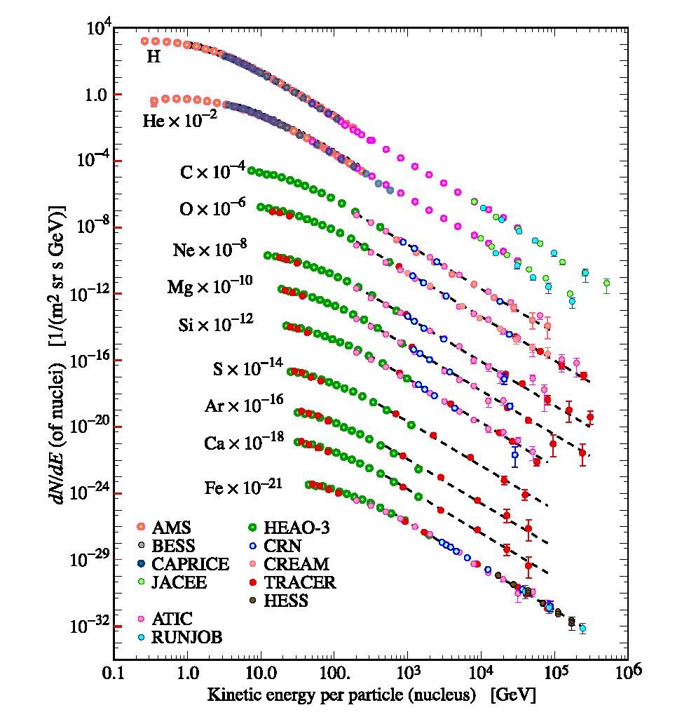
$$ I(E) \approx 1.8 \times 10^4 (E/1\; \rm{GeV})^{-2.7} \frac{\rm{nucleons}}{\rm{m}^2\; \rm{s\;sr\;GeV}}$$
Where $\alpha \equiv 1+ \gamma = 2.7$ is the differential spectral index. Free protons are about ~79%. He is 15%. The rest are heavier nuclei: C, O, Fe and other ionized nuclei and electrons (2%)
Galactic Cosmic Ray Composition
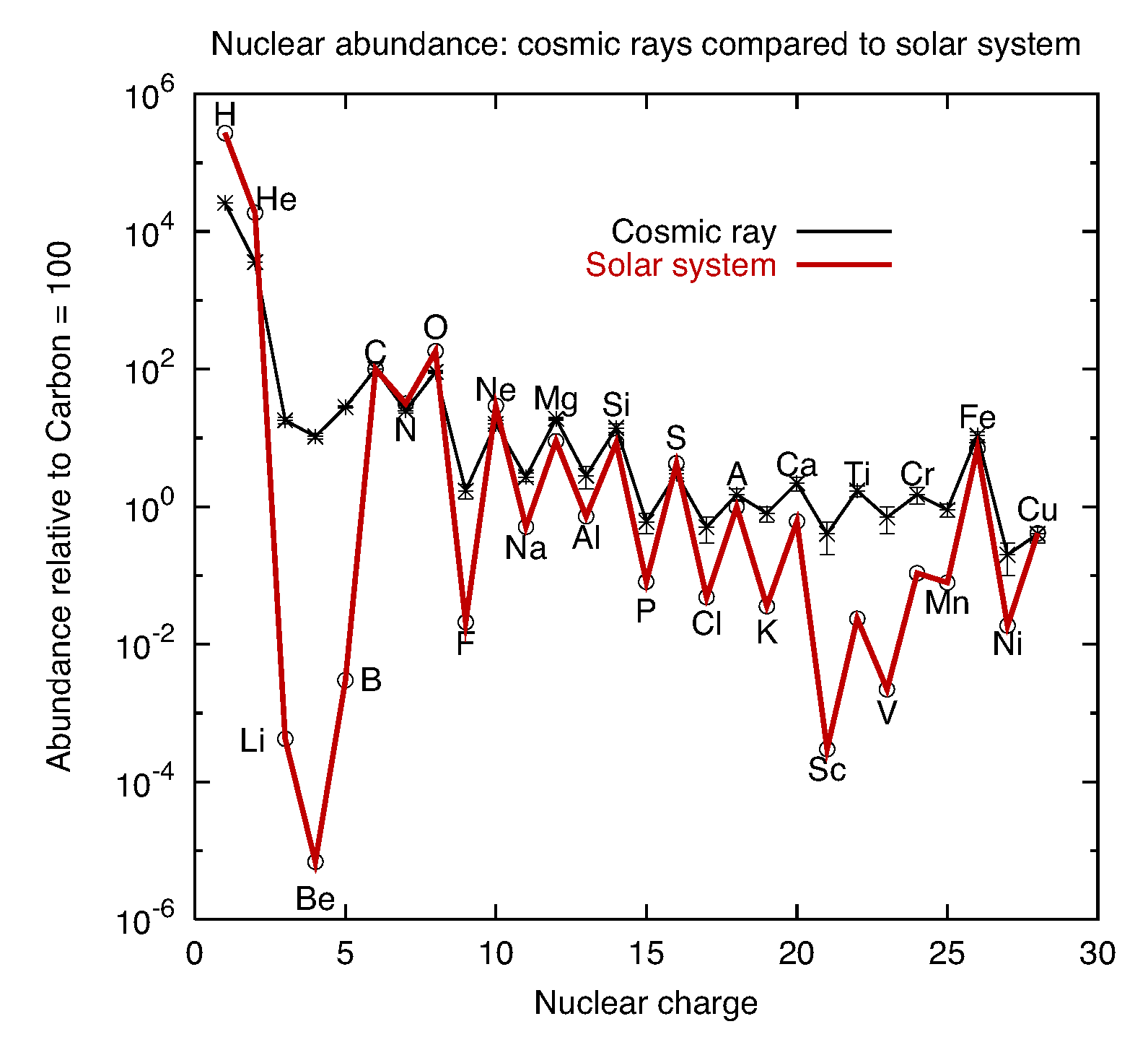
- The chemical composition of cosmic rays is similar to the abundances of the elements in the Sun indicating an stellar origin of cosmic rays.
- However there are some differences: Li, Be, B are secondary nuclei produced in the spallation of heavier elements (C and O). Also Mn, V, and Sc come from the fragmentation of Fe. These are usually referred as secondary cosmic rays.
- The see-saw effect is due to the fact that nuclei with odd Z and/or A have weaker bounds and are less frequent products of thermonuclear reactions.
By measuring the primary-to-secondary ratio we can infer the propagation and diffusion processes of CR
Electrons
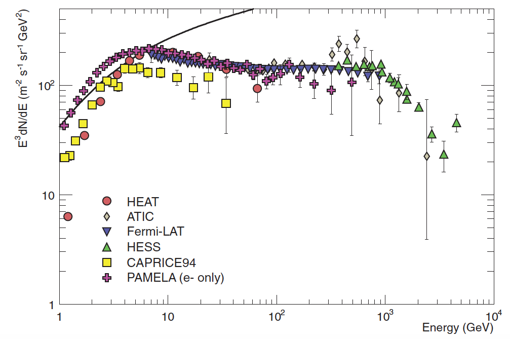
- The spectrum of electrons is expected to steepen by one power of E at around ~5 GeV because the radioactive energy loss in the galaxy.
- The proton spectrum is also shown multiplied by 0.01.
- ATIC measured and excess at 600 GeV while HESS measured a cutoff at ~ 1 TeV but no evidence for an excess.
Question
Assuming the electron flux is only 1% of the protons. Is it the Earth positive charged-up?Electron to positron ratio
- As antimatter is rare in the Universe today, all antimatter we observe are by-product of particle interactions such as Cosmic Rays interacting with the interstellar gas.
- The PAMELA and AMS-02 satellite experiments measured the positron to electron ratio to increase above 10 GeV instead of the expected decrease at higher energy.
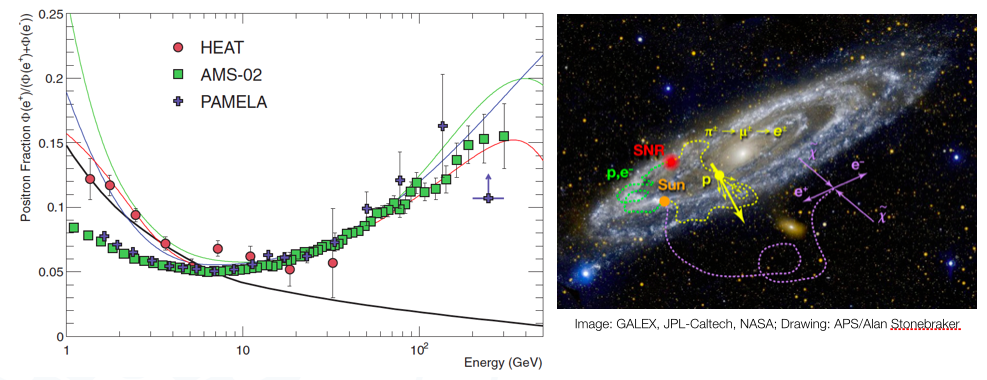
This excess might hint to to contributions from individual nearby sources (supernova remnants or pulsars) emerging above a background suppressed at high energy by synchrotron losses
Dynamic of charge particles in magnetic fields.
The galactic CR flux is, to some extent very isotropic. On the other hand, their sources should be mainly distributed on the Galactic Plane. That means that CRs undergo a diffusion process due to the magnetic field lines in the Galaxy.
Let's assume the simplest case of a test particle or mass $m_0$ and charge $Ze$ and lorentz factor $\gamma$ in an uniform static magnetic field, ${\bf B}$.
$$\frac{d}{dt}(\gamma m_0 {\bf v}) = Ze ( {\bf v} \times {\bf B})$$knowing the expression of $\gamma$ we derive this:
$$m_0 \frac{d}{dt}(\gamma {\bf v}) = m_0\gamma\frac{d{\bf v}}{dt} + m_0\gamma^3{\bf v}\frac{{\bf v\cdot a}}{c^2}$$In a magnetic field the acceleration is always perpendicular to ${\bf v}$ so ${\bf v\cdot a} = 0$ resulting in:
$$m_0\gamma\frac{d{\bf v}}{dt} = Ze ( {\bf v} \times {\bf B})$$This equation tell us that there is no change in the $v_{\parallel}$ the parallel component of the velocity and the aceleration is only perpendicular to the magnetic field direction, $v_{\perp}$. Beacuse ${\bf B}$ is constant this results in a spiral motion around the magnetic field.
Motion of a charge particle in a slowly changing magnetic field
q = 1.0
m = 1.0
dt = 1e-3
t0 = 0
t1 = 10

t = linspace(t0, t1, (t1 - t0)/dt)

n = len(t)
print "Number of elements in t array: ", n

r = zeros((n,3))
v = zeros((n,3))

#Initial conditions

r[0] = [0.0, 0.0, 0.0]
v[0] = [2.0, 0.0, 3.0]

#B = array([0.0, 0.0, 5.0])

B = zeros((n,3))
B[0] = array([0.0, 0.0, 5.0])
dB = array([0.0, 0.0, 1e-3])
for i in range(len(t)-1):
    a   = q/m* cross(v[i],B[i])
    v[i+1] = v[i] + a*dt
    r[i+1] = r[i] + v[i+1]*dt
    B[i+1] = B[i] + dB
from mpl_toolkits.mplot3d import Axes3D

figure(figsize=(12,10))
ax = gca(projection='3d')
plot(r[:,0], r[:,1], r[:,2])

ax.set_xlabel("$x$",fontsize=26)
ax.set_ylabel("$y$",fontsize=26)
ax.set_zlabel("$z$",fontsize=26)

Dynamic of charge particles in magnetic fields.
The previous picture is a very simplistic one. Magnetic fields can vary slowly in time and have turbulences. In addition, generally cosmic ray particles propagate in collisionles, high-conductive, magnetized plasma consisting mainly of protons and electrons. Very often the energy density of cosmic ray partciles is comparable to that of the background medium and as a consequence, the electromagnetic field in the system is severely influenced by the cosmic ray particles and the description is more complex than the motion of a test charged particle in a fixed electromagnetic field.
Cosmic-ray interactions.
Cosmic-ray particles are expected to interact during their travel.
- Coulomb collissions: They occur when a particle interacts with another particle via electric fields.
- The Coulomb cross-section for a 1 GeV particle is 10$^{-30}$ cm$^2$
- For 1 GeV cosmic-ray propating in the ISM (n $\sim$ 1 cm$^{-3}$) the mean Coulomb collision rate is $n\sigma v \sim 10^{-19.5} {\rm s}^{-1}$ which corresponds to 1% in a Hubble time! $\rightarrow$ Coulomb collisions can be neglected.
- Spallations processes: It occurs when C, N, O, Fe nuclei impact on intestellar hydrogen.
- The large nuclei is broken up into smaller nuclei.
Primary-to-Secondary ratios
Since we know the partial cross-section of spallation processes we can use the secondary-to-primary abundance ratios to infer the gas column density traversed by the average cosmic ray.
Let us perform a simply estimate of the Boron-to-Carbon ratio. Boron is chiefly produced by Carbon and Oxygen with approximately conserved kinetic energy per nucleon (see Superposition principle), so we can relate the Boron source production rate, $Q_B(E)$ to the differential density of Carbon by this equation:
$$Q_B(E) \simeq n_{H} \beta c \sigma_{\rightarrow B} N_C$$where, $n_H$ denotes the average interstellar gas number density and $N_C$ is the Carbon density and $\beta c$ is the Carbon velocity and $\sigma_{\rightarrow B}$ is the spallation cross-section of Carbon into Boron.
The Boron density is related to the production rate by the lifetime of Boron in the Galaxy, $\tau$, before it escapes or losses itself energy by spallation:
$$Q_B = \dot{N}_B = \frac{N_B}{\tau}$$where we used $\dot{N}_B = \frac{N_B}{\tau}$ assuming a constant per unit time lifetime (see next Leaky Box model). So we can write:
$$\frac{N_B}{N_C} \simeq n_{H} \beta c \sigma_{\rightarrow B}\tau$$Boron-To-Carbon ratio
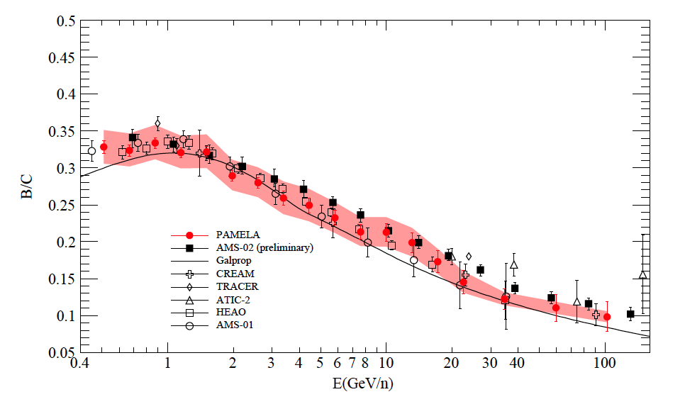
Above about 1 GeV/nucleon the experimental data can be fitted to a test function $\mathcal{f} = 0.4\beta E^{-0.3}$, therefore the Boron-to-Carbon ratio can be expressed as:
$$\frac{N_B}{N_C} = n_{H}\beta c \sigma_{\rightarrow B} \tau =0.4\beta E^{-0.3}$$which leads, using the values of the cross-section, to a life time gas density of:
$$ n_H \tau \simeq 10^{14}\left(\frac{E}{\rm{GeV}}\right)^{-0.3} \; \rm{s}\;\rm{cm}^{-3} $$Boron Lifetime
But what is this Boron lifetime? The lifetime $\tau$ for Boron includes the catastrophic loss time due to the partial fragmentation of Boron, $\tau_{f,B}$ and the escape probability from the Galactic confinement volume, $T_{esc}$. The fragmentation cross section is $\sigma_{f,B} \approx 250$ mbarn so we find that:
$$n_H \tau_{f,B} = \frac{n_H}{n_H \beta c \sigma_{f,B}} \simeq 1.4 \times 10^{14}\; \rm{s}\;\rm{cm}^{-3} $$which is larger than the total lifetime, so there must be another loss process $T_{esc}$. By summing the inverse of these processes (being exponential processes):
$$\tau^{-1} = n_H \beta c \sigma_{f,B} + T^{-1}_{esc}$$and solving for $T_{esc}$ we have that:
$$n_H T_{esc} = \frac{n_H}{\frac{1}{\tau} - \frac{1}{\tau_{f,B}}} \simeq \frac{10^{14} \; \rm{s}\;\rm{cm}^{-3}}{\left(\frac{E}{\rm{GeV}}\right)^{-0.3} -0.7} \simeq 10^{14}\left(\frac{E}{\rm{GeV}}\right)^{-0.55} \mbox{ for 3}\leq \frac{E}{\rm{GeV}} \leq 20$$The Leaky Box model
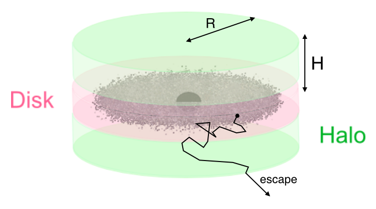
In the above calculation we used some assumptions based on the so-called Leaky Box model. This is a very simple model used to describe CR confinement.
In this simplified phenomenological picture CRs are assumed be accelerated in the galactic plane and to propagate freely within a cylindrical box of size $H$ and radius $r$ and reflected at the boundaries; the loss of particles is parametrized assuming the existence of a non-zero probability of escape for each encounter with the boundary (Poisson process).
Diffusion
The equation that we used to relate the Boron production rate by the Carbon spallation process can be seen aa a diffuse equation.
In diffusion the continuity equation states that the variation of the density $N$ in time is given by its transfer of flux in area plus the source contribution:
$$\frac{\partial N}{\partial t}= - \nabla \cdot \mathbf{J} + Q $$where $Q$ is intensity of any local source of this quantity and $\mathbf{J}$ is the flux.
Fick's first law: the diffusion flux is proportional to the negative of the concentration gradient in an isotropic medium:
$$\mathbf{J}=-D \nabla N \ , \;\; J_i=-D \frac{\partial N}{\partial x_i} \ $$where the proporcionality constant is called diffusion coefficient. Which leads to the diffusion equation of:
$$\frac{\partial N}{\partial t}= \nabla^2 \cdot \mathbf{J} + Q = \Delta \mathbf{J} + Q $$where $\Delta$ is the Laplace operator.
The Leaky Box model
In the Leaky Box model the diffusion equation, ignoring other effects, can be written as:
$$\frac{\partial N_i}{\partial t} = D\Delta N_i =-\frac{N_i}{T_{esc}}$$where we made use of the fact that the escape probability is constant per unit time (Poisson process) and so the disitribution in time can be writen as: $N_i(t) = n_0 exp(−t/T_{esc})$
In the equation above $D$ is the diffusion coefficient and $\Delta$ is the Laplace operator. Without diffusion the $T_{esc}$ will be H/c which is the time required by CR generated in the Galactic plane to escape the box of height $H$. However we know that $T_{esc} \gg H/c$ so there must be diffusion. In the absent of collisions and other energy changing processes, the distribution of cosmic ray path lengths can be written as $N_i = n_0 exp(−t/T_{esc}) = n_0 exp(−z/H)$ so we can use the diffusion equation to write:
$$T_{esc} = \frac{H^2}{D} \rightarrow D(E) \propto E^{\delta} \sim E^{0.55}$$The state-of-art of Diffusion
The leaky box model is a very simplistic approximation but more realistic diffusion models, such as the numerical integration of the transport equation in the GALPROP code (Strong and Moskalenko 1998), lead to results for the major stable cosmic-ray nuclei, which are equivalent to the Leaky-Box predictions at high energy. However sofisticated models of transport should include effects such as:
- Diffusion coefficient non spatially constant.
- Anisotropic diffusion (Parallel vs Perpendicular)
- Effect of self-generation waves induced by CR.
- Damping of waves and its effects in CR propagation
- Cascading of modes in wavenumber space
Each of these effects might change the predicted spectra and CR anisotropies in significant ways.
Transport equation on Primaries
The general simplified transport/dissusion equation that relate the abundances of CR elements can be given by:
$$\frac{\partial N_i(E)}{\partial t} =\frac{N_i(E)}{T_{esc}(E)} = Q_i(E) - \left(\beta c n_H \sigma_i + \frac{1}{\gamma\tau_i}\right)N_i(E) + \beta c n_H \sum_{k\ge i}\sigma_{k\rightarrow i}N_K(E)$$where now $Q_i(E)$ is the local production rate by a CR accelerator, the middle part reprensents the losses due to interactions with cross-section $\sigma_i$ and decays for unestable nuclei with lifetime $\tau_i$. The last term is the feed-down production due to spallation processes of heavier CR. We can simplified this equation depending if we are dealing with Primary or Secondary CR:
- Primaries $\rightarrow$ neglect spallation feed-down.
- Secondaries $\rightarrow$ neglect production by sources: $Q_s = 0$
For example, let's assume now a primary CR, $P$, where feed-down spallation is not taking place (ie, they are not product of heavier CR) and no decay (most nuclei are stable, one exception is $^{10}$Be which is unstable and $\beta$-decay), the equation can be written as:
$$\frac{N_P(E)}{T_{esc}(E)} = Q_P(E) - \frac{\beta c \rho_H N_P(E)}{\lambda_P(E)} \rightarrow N_P(E) = \frac{Q_P(E)}{\frac{1}{T_{esc}(E)}+\frac{\beta c \rho_H}{\lambda_P(E)}}$$where we wrote $n_H = \rho_H/m$ and $\lambda_P$ is the mean free path in g / cm$^2$.
Transport equation on Primaries
While $T_{esc}$ is the same for all nuclei with same rigidity, $\lambda_i$ is different and depends on the mass of the nucleus. The equation suggests that at low energies the spectra for different nuclei will be different (eg for Fe interaction dominates over escape) and will be parallel at high energy if accelerated on the same source.
$$N_{p}(E) = Q_p(E)\cdot T_{esc}(E)$$
ie, we observe at Earth a proton density of $N_p(E)\propto E^{\gamma + 1} \sim E^{2.7}$ at the production site it must be $Q_p(E) \propto E^{\alpha}$ with
$$\alpha = (\gamma + 1) -\delta \approx 2.1$$
Energy density of galactic CR
The flux, $\mathcal{F}$, of CR from one hemisphere on a planar detector is connected to the spectrum $I(E)$ by:
$$\begin{align*} \mathcal{F}(E) &= \int {\rm d}\Omega I(E) \cos\theta = I(E) \int_0^{2\pi}{\rm d}\Phi \int_0^{\pi/2}{\rm d}\theta \sin\theta \cos\theta\\ &= \pi I(E) \int_0^{\pi/2} {\rm d}\sin\theta\cos2\theta = \pi I(E) \end{align*}$$The number density of CR with velocity $v$ is given by $n(E) = \frac{4\pi}{v}I(E)$
And so kinetic energy density of CR, $\rho_{CR}$ is therefore the integral of the energy density flux, $E\cdot n(E)$:
$$\rho_{CR} = \int E n(E) {\rm d} E =4\pi \int \frac{E}{v}I(E) {\rm d} E$$assuming for the Galactic CR:
$$ I(E) \approx 1.8 \times 10^4 (E/1\; \rm{GeV})^{-2.7} \frac{\rm{nucleons}}{\rm{m}^2\; \rm{s\;sr\;GeV}}$$the integral gives $\rho_{CR} \approx 0.8$ eV/cm$^{3}$ which is comparable with the energy density of the CMB $\rho_{CMB} \approx 0.25$ eV/cm$^{3}$
Power required for galactic CR
If we assume this value to be the constant value over the galaxy, the power required (called luminosity in astrophysics) to supply all the galactic CR and balance the escape processes is:
$$\mathcal{L}_{CR} = \frac{V_D \rho_E}{\tau_{esc} }\sim 5\times 10^{40} {\rm erg\;s}^{-1}$$where $V_D$ is the volume of the galactic disk
$$V_D = \pi R^2 d \sim \pi (15 {\rm kpc})^2(200 {\rm pc}) \sim 4 \times 10^{66} {\rm cm}^3.$$It was emphasized long ago (Ginzburg & Syrovatskii 1964) that supernovae might account for this power. For example a type II supernova gives an average power output of:
$$\mathcal{L}_{SN} \sim 3 \times 10^{42} {\rm erg\;s}^{-1}$$Therefore if SN transmit a few percent of the energy into CR it is enough to account for the total energy in the cosmic ray beam $\rightarrow$ SNR paradigm
Power required for > 100 TeV
The derivation above was considered using the CR flux with an integral spectral index of $\gamma = \alpha -1 = 1.7$ which describes well the CR up to the knee. This is the bulk of cosmic ray density. The power required for the high energy part will be significantly less due to the steeply falling primary cosmic ray spectrum. For example assuming an integral index of $\gamma = 1.6$ for $E < 1000$ TeV and $\gamma = 2$ for higher energy we get:
$$\begin{align*} \sim 2 \times 10^{39} {\;\rm\;erg/s\; for\; } E &> 100 {\rm\; TeV}\\ \sim 2 \times 10^{38} {\;\rm\;erg/s\; for\; } E &> 1 {\rm\; PeV}\\ \sim 2 \times 10^{37} {\;\rm\;erg/s\; for\; } E &> 10 {\rm\; PeV} \end{align*}$$which are considerably less than the total power required for all the cosmic-rays. This power might be available from a few very energetic sources.
Fermi Mechanism
Fermi studied how it is posible to transfer macroscopic kinetic energy of moving magnetized plasma to individual particles. He considered an iterative process in which for each encounter a particle gains energy which is proportional to the energy.
Let's write the increase in energy as $\Delta E = \xi E$ after $n$ encounters then:
$$E_n = E_0(1 + \xi)^n$$where $E_0$ is the injection energy in the acceleration region. If the probability of escaping this acceleration region is $P_{esc}$ per encounter, after $n$ the remaining probability is $(1 - P_{esc})^n$. To reach a given energy $E$ we need:
$$n = {\rm In}\left(\frac{E}{E_0}\right)/{\rm In}(1 + \xi)$$the proportion of particles with energies greater than $E$ will be:
$$N(\ge E) \propto \sum_{m = n}^{\infty} ( 1- P_{esc})^m $$using that $\sum_{0}^{\infty}x^m = \frac{1}{1-x}$ for $x < 1$ we can write:
$$N(\ge E) = (1 - P_{esc})^n \sum_{m = n}^{\infty} ( 1- P_{esc})^{m - n} = (1 - P_{esc})^n \sum_{m = 0}^{\infty} ( 1- P_{esc})^{m}= \frac{(1 - P_{esc})^n}{P_{esc}}$$replacing the first in the second and using $x^{log y} = y^{log x}$:
$$N(\ge E) \propto \frac{1}{P_{esc}} \left(\frac{E}{E_0}\right)^{-\gamma}$$with
$$\gamma = {\rm In}\left(\frac{1}{1+P_{esc}}\right)/{\rm In} (1+\xi) \approx \frac{P_{esc}}{\xi} = \frac{1}{\xi}\cdot\frac{T_{cycle}}{T_{esc}}$$where $T_{cycle}$ is the characteristic time of acceleration cycle, and $T_{esc}$ is the characteristic time to escape the accelarion region.
Fermi Mechanism
A mechanism working for a time $t$ will produce a maximum energy: $$E\leq E_0 (1+\xi)^{t/T_{cycle}}$$
Two characteristic features are apparent from this equation:
- High energy particles take longer to accelerate
- If a given kind of Fermi accelerator has a limited lifetime this will be characterize by a maximum energy per particle that can produce.
Fermi Mechanism
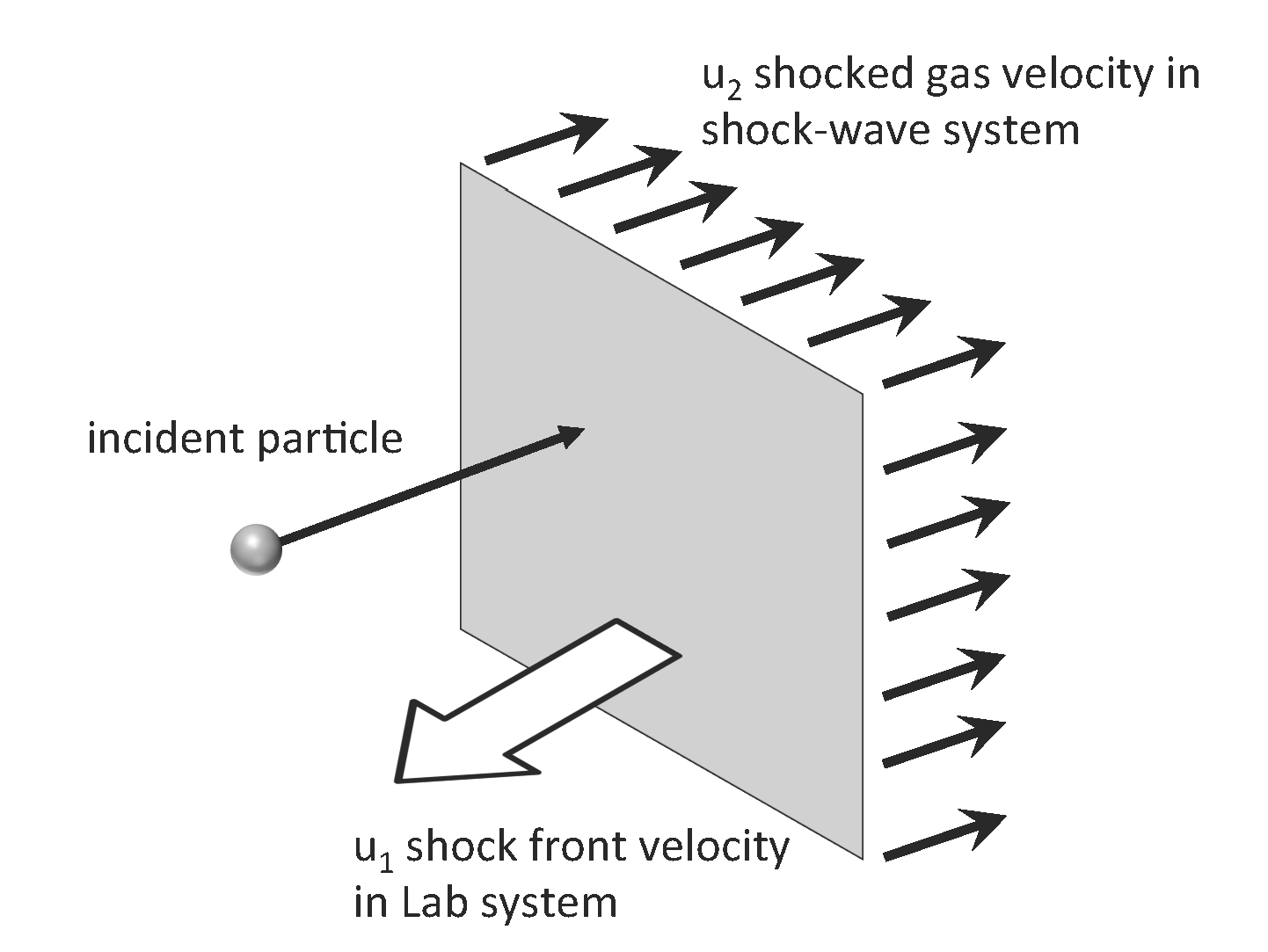
Simple model
A particle of velocity $v$ collides perpendicularly with a shock front $u_1$. Behind the shock the gas recedes at a speed $u_2$ so in the lab frame the gas has a recesing speed of $u_1 - u_2$. As the particle is reflected back it gains the kinetic energy of the shocked gas. The kinetic energy gain is:
Assuming $v \gg u_1, u_2, u_1 > u_2$ then:
$$\frac{\Delta E}{E}\approx \frac{2(u_1 - u_2)}{v}$$
Fermi Acceleration
1st and 2nd order model
This was a simplified version where only perpendicular and non-relativistic particle interact with a shock wave. In the general approach, the particle might enter the shock or some other "encounter" such as a magnetic cloud, at different angles and exit at difference angles. In the rest frame of the moving gas, a particle with energy $E_1$ hast a total energy of:
$$E_1^\prime = \gamma E_1 (1 -\beta \cos\theta_1)$$Before leaving the gas cloud the particle has an anegy $E_2^\prime$. If we transform this back to the lab reference system we get:
$$E_2 = \gamma E_2^\prime (1 +\beta \cos\theta_2^\prime)$$where primes denote the values measured in the rest frame of the cloud and $\beta$ refers to the plasma flow (not the CR). As the particle suffers from colissioness scatterings inside the cloud the energy in the moving frame just before it escapes is $E_2^\prime = E_1^\prime$ and so:
$$\frac{\Delta E}{E_1} = \frac{1 - \beta \cos \theta_1 + \beta\cos\theta_2^\prime - \beta^2\cos\theta_1\cos\theta_2^\prime}{1 - \beta^2} -1$$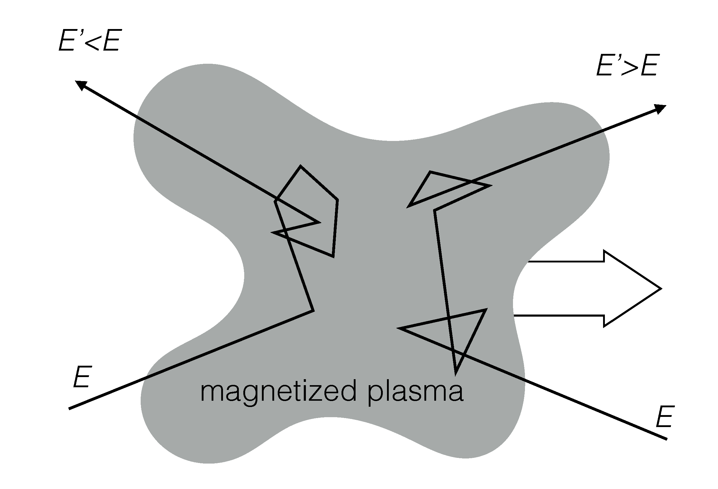
The scattered angle is uniform so the average value is $\langle \cos\theta_2^\prime\rangle = 0$.
The probability of collision with the cloud is proportional to the relative velocity between the cloud and the particle:
and so:
$$\langle \cos\theta_1\rangle = \frac{\int \cos\theta_1 \cdot \frac{dn}{d\cos\theta_1} d\cos\theta_1}{\int \frac{dn}{d\cos\theta_1}d\cos\theta_1} = - \frac{\beta}{3}$$Particles can gain or lose energy depending on the angles, but on average the gain is $$\xi = \frac{1 + \frac{1}{3}\beta^2}{1 - \beta^2} \sim \frac{4}{3}\beta^2$$
Fermi Acceleration
Problems with the 2nd order acceleration
- The energy increase is second order of $\beta$ and..
- ... the random velocities of clouds are relatively small: $\beta \sim 10^{-4}$ !!!
- Some collisions result in energy losses! Only with the average one finds a net increase.
- Very little chance of a particle gaining significant energy!
- The theory does not predict the power law exponent
Fermi Acceleration
1st order acceleration.
- In the first order a shock front moves with speed $-\vec{u_1}$. The shocked gas flows away from the shock with a velocity ${\vec u_2}$ where $|u_2| < |u_1|$. In the lab frame the gas moves left with speed ${\vec V = - \vec u_1 + \vec u_2}$ and $\beta = V/c$ refers now to the shocked (downstream) gas.
- The distribution of encounters is the projection of an uniform flux on a plane:
which gives:
$$\langle \cos\theta_2^\prime\rangle = \frac{\int \cos\theta_2^\prime \cdot \frac{dn}{d\cos\theta_2^\prime} d\cos\theta_2^\prime}{\int \frac{dn}{d\cos\theta_2^\prime}d\cos\theta_2^\prime} = \frac{2}{3}$$- The incoming angle distribution is also the projection of an uniform flux on a plen but this time with $-1 \leq \cos\theta_1 \leq 0$ and so $\langle \cos \theta_1 \rangle = -2/3$
Particles entering the shockwave and exiting will have a gain of:
$$\xi = \frac{1 + \frac{4}{3}\beta + \frac{4}{9}\beta^2}{1 -\beta^2} - 1 \sim \frac{4}{3}\beta = \frac{4}{3}\frac{u_1 - u_2}{c}$$- Incoming flux. The rate of encounters for a plane shock is the projection of an isotropic flux onto the plane shock:
where $n(E)$ is the CR number density.
- Outgoing flux. In the shock rest frame, there is an outflow of cosmic-rays upstram given simply by $\Phi_{out} = n(E) u_2$,
Therefore the escape probability is given by:
$$P_{esc} = \frac{\Phi_{in} }{\Phi_{out} }= \frac{4 u_2}{c}$$which for acceleration at shock gives:
$$\gamma = \frac{P_{esc}}{\xi} = \frac{3}{u_1/u_2 -1}$$So we get an estimate of the spectral index based on the relative velocities of the downstream and upstram gas in the sockwave.
Kinematic relations at the shock
In order to derive the exact value of the spectral index we need to obtain a relation between $u_1$ and $u_2$ using the kinematics of a shock wave. This equations are the conservation of mass, the Euler equation for momentum conservation and conservation of energy:
Conservation of mass: $$\partial_t \rho + \nabla \cdot (\rho\vec{u}) = 0$$
Conservation of momentum (Euler equation):
where $\vec{F}$ is an external force, and $\nabla P$ is a force due to a pressure gradient.
- Conservation of energy:
where this equation accounts for the kinetic, internal, and potential energy $\Phi$.
Let's assume a one-dimensional, steady shoch in its rest frame. Then the first equation becomes simply:
$$\frac{d}{dx} (\rho u) = 0$$and the Euler equation simplifies to:
$$\frac{d}{dx}(P + \rho u^2) = 0$$In the energy equation we assune $\Phi = 0$:
$$\frac{d}{dx}\left(\frac{\rho u^3}{2} + (\rho U + P)u\right) = 0 $$where U is the internal density per unit volume and we can write $\rho U = P /(\Gamma -1)$, where $\Gamma = c_p/c_v$ is the adiabatic index or heat capacity ratio.
Condition at the discontinuity of the shock wave
Applyting these equations at the discontinuity of the shock we have:
$$\begin{align*} \rho_1 u_1 &= \rho_2 u_2\\ P_1 + \rho_1 u_1^2 &= P_2 + \rho_2 u_2^2\\ \frac{\rho_1 u_1^3}{2} + \frac{\Gamma}{\Gamma - 1} P_1 u_1 &=\frac{\rho_2 u_2^3}{2} + \frac{\Gamma}{\Gamma - 1} P_2 u_2\\ \end{align*}$$Using these expression ot eliminate $\rho_2$ and $P_2$ we have:
$$\frac{\Gamma + 1}{\Gamma -1} u_2^2 + \frac{2\Gamma}{\Gamma -1} \left(\frac{P_1 + \rho_1 u_1^2}{\rho_1 u_1}\right)u_2 + v_1^2\frac{2\Gamma}{\Gamma - 1}\frac{P_1}{\rho_1} = 0$$using the fact that pressure is related to the spead of sound as $\rho c_s^2 = \Gamma P$ and the Mach number $\mathcal{M} = u/c_s$ we can rewrite by dividing by $v_1$ and defining $t = u_2/u_1$:
$$\frac{\Gamma + 1}{\Gamma -1} t^2 + \frac{2\Gamma}{\Gamma -1} \left(\frac{1}{\mathcal{M}^2} + \Gamma\right) t + \left( 1 + \frac{1}{\mathcal{M}^2}\frac{2}{\Gamma - 1}\right) = 0$$For strong waves $\mathcal{M} \gg 1$ we can ignore the terms $1/\mathcal{M^2}$ and the the quadratic equation has the 2 solutions: $$ t = 1 \rightarrow u_1 = u_2$$
and:
$$ t = \frac{\Gamma - 1}{\Gamma + 1} \rightarrow \frac{u_2}{u_1} = \frac{\Gamma - 1}{\Gamma +1}$$for a monoatomic gas the ratio of specific heats is $\frac{5}{3}$, so
$$\frac{u_2}{u_1} = \frac{1}{4}$$No matter how strong a shock wave is, a mono-atomic gas can only be compressed by a factor of 4. The spectral index is then:
$$\gamma = \frac{P_{esc}}{\xi} = \frac{3}{u_1/u_2 -1} = 1$$If one keeps the factors of $1/\mathcal{M}^2$:
$$\gamma \sim 1 + \frac{4}{\mathcal{M}^2} \sim 1.1$$Which matches remarkably to what we derived to be the differential spectral index at the accelerator ${\rm d}N/{\rm d}E \propto E^{-(\gamma+1)} \sim E^{-2.1} $
Maximum Energy
The maximum energy we can get with Fermi mechanism is limited by the timelife of the shockwave. The resulting estimate of the maximum energy is (not derived here):
$$E_{max} \leq \frac{3}{20}\frac{u_1}{c} Z e B (u_1 T_A)$$where $T_A$ is the time in which the accelerator is working. Using some estimates on the time ($T_A \sim$ 1000 yrs as the typical SN shockwave) and $B_{ISM} \sim 3 \mu$Gauss then gives:
$$E_{max} \leq Z\times 3 \times 10^4 {\rm GeV}$$In order words, the shock-wave acceleration shown can accelerate CR up to 100 Z TeV, but not beyond this. Other acceleration mechanism are needed for the highest energy cosmic rays. We need very high magnetic fields (non-lineal acceleration mechanism). In these cases, even if this object cannot supply the all the galactic cosmic rays the energy per particle may be orders of magnitude higher than those possible in shock acceleration by blast waves.
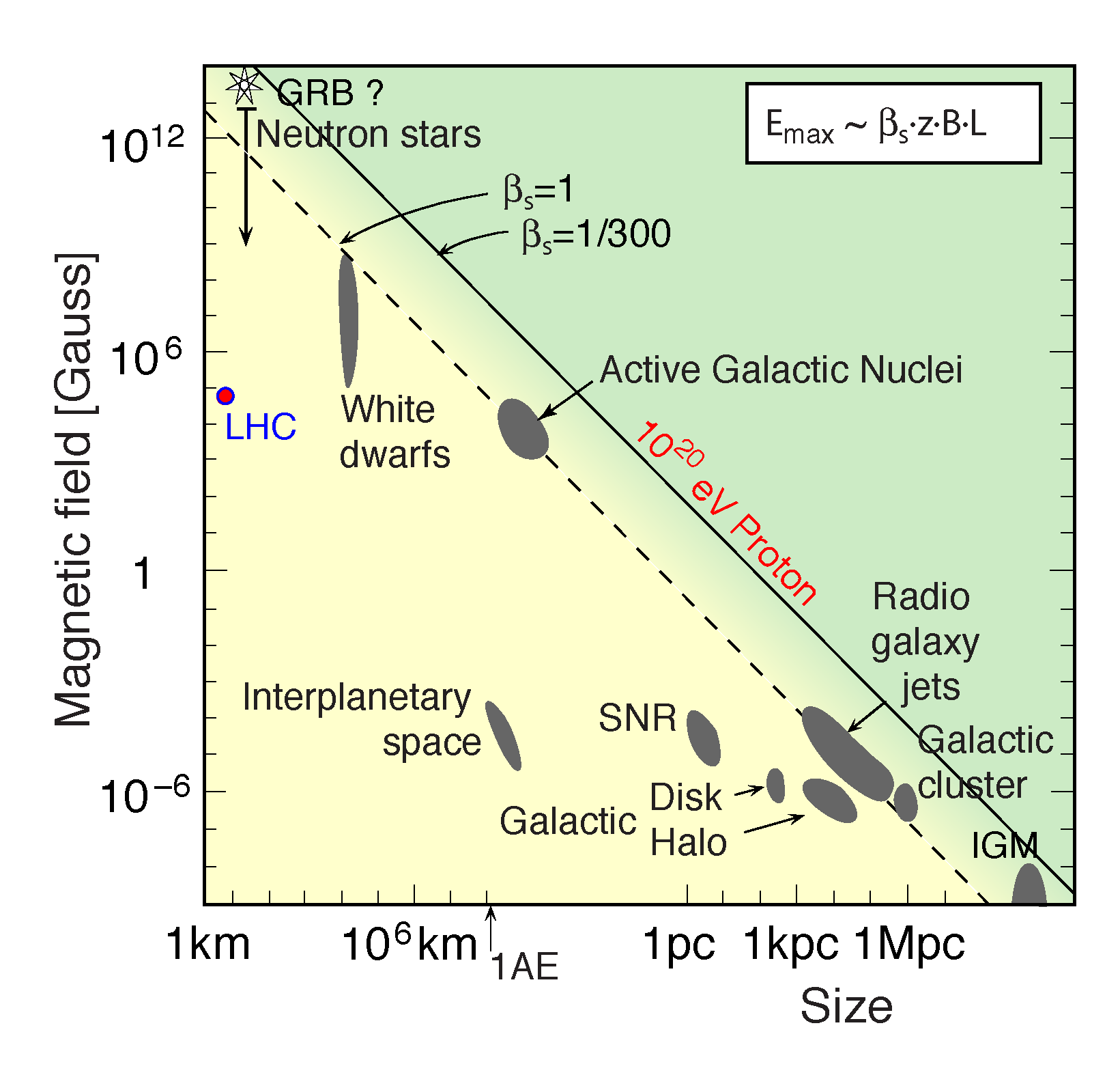
Hillas Plot
Supernova Remnants (SNRs)
Supernova remnants (SNR) remain the most likely candidates for CR acceleration up to at least 10$^{14}$ eV via the Fermi shock mechanism. Supernova explosions are very violent events which transfer a significant amount of energy in the ISM. The explosion mechanism can be the carbon deflagration of white dwarts (Type I) or the core collapse of masssive stars (Type II) but the dynamical evolution of the supernova remnant (SNR) i.e., the expanding cloud of hot gas in the ISM is similar:
Free Expansion Phase. The shock wave moves in the ISM gas a highly supersonic speed. The shock radious scalase as: $R_s(t) = v_e t$. Behind the shockfront ISM gas starts to accumulate an a reverse shock starts to form. Sometimes we see first this reverse shock. At some point the compressed ISM gas equals the ejected material, this marks the ned of the free expansion phase. It lasts less than 200-300 years.
Sedov-Taylor Phase. Once the reverse shock reaches the nucleus, the interior of the SNR gets very hot that energy losses due to radiation are not possible (all atmos are ionized). The cooling of the gas is only due to the expansion, that's why this phase is the adiabatic phase. The radius goes as $R \propto t^{2/5}$. When temperature reaches the critical value of $10^{6}$ K ionized atoms start to capture free electrons and can lose energy due to de-exitation. This is the end of the adiabatic phase. This phase can last 20,000 years. This is the phase when Cosmic Rays are mostly accelerated.
Cooling or Snowplough phase Due to the effective radiative cooling the thermal presure decreases and the expansion slows down. More and more interstellar gas is accumulated until the swept-up mass is much larger than the ejected material. Finally the shell breaks up into clumps probably due to Rayleigh-Taylor inestabilities. This phase lasts up to 500,000 years.
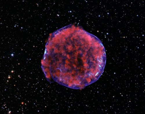
The Tycho SNR
Other sources of Galactic Cosmic Rays
Neutron stars Neutron stars, especially young fast-rotating pulsars and magnetars possess extreme magnetic fields (up to 10$^{12}$ G in the case of magnetars) with complex structure that could accelerate CR up to the highest energies. These objects are far rarer than SNRs, however, only a dozen magnetars are known in the Milky Way, although many could exist in the local neighborhood.
Microquasars are radio-intense X-ray binary stars with companion orbiting an accreting black hole. They are particularly interesting particle accelerators due to observation of VHE gamma ray emission and highly relativistic jets which could provide energy for UHECR
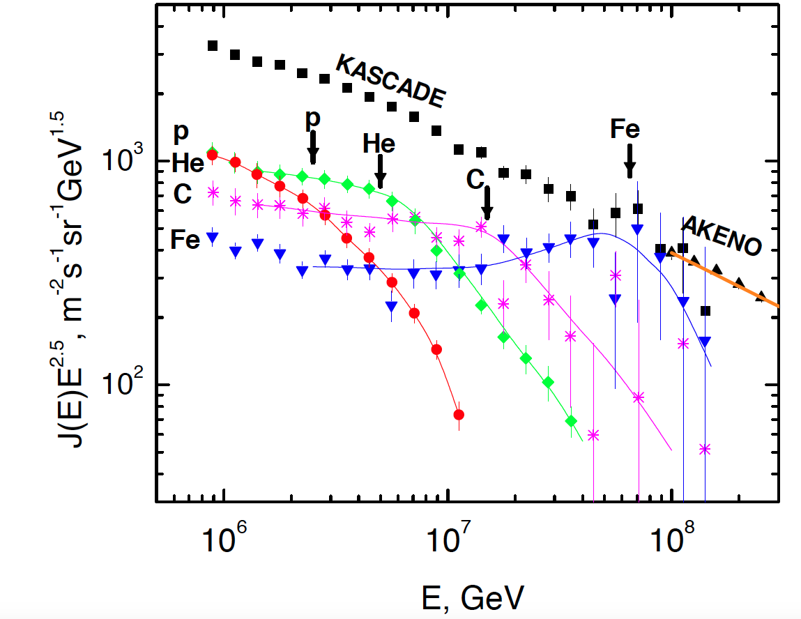
The Knee
- At energies of about 5 $\times 10^{15}$ eV a steepening in the spectrum from $\gamma \sim 1.7 \rightarrow \gamma \sim 2$ known as the knee takes place.
Alread Peters in 1959 concluded that it could be due to:
- Consequence of the breakdown of an acceleration mechanism.
- Increased rate of escape from the galaxy at high energies.
A third explanation could be a change in CR interactions at ${\sqrt s} \sim $ few TeV. The first two explanantions produce a rigidity dependent knee, ie the position of the knee for different nuclei depends on $Z$, while the third explanation will depend on $A$.Experimentally the rigidity dependence is favored.
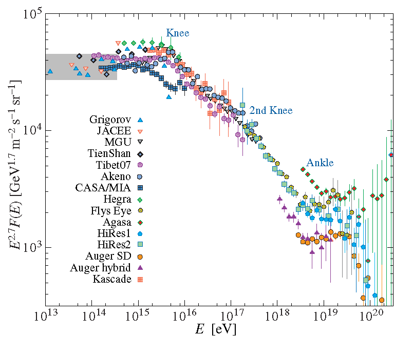
The Ankle and beyond
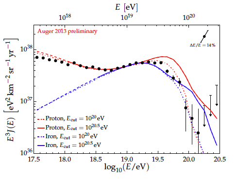
- A proton of energies $10^{18}$ eV has a gyroradious of a kpc in a typical magnetic field $\rightarrow$ extra-Galactic origin.
- Greissen-Zatsepin and Kuz-min predicted that at energies of $\sim 10^{19}$ eV will interact with the low energy photons of the CMB. This interaction leads to a supression of flux above $5\times10^{19}$ eV unless the sources are within a few tens of Mpc. This supression is referred as GZK cutoff.
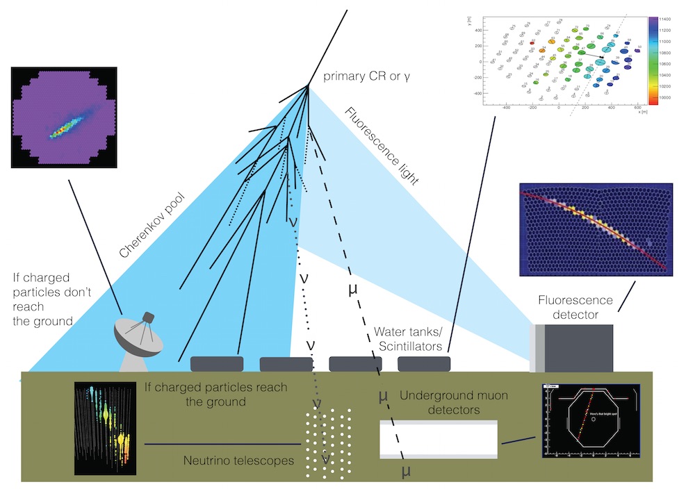
Detection of UHECR
Electromagnetic cascades and air showers
Ionization losses
The ionization energy loss of high energy charged particles with colission with atomic electrons is given by the Bethe-Block formula:
$$\left(\frac{{\rm d} E}{{\rm d} x}\right)_{ion}= -\left(\frac{4\pi N_0z^2e^4}{mv^2}\right)\left(\frac{Z}{A}\right)\left\{{\rm In}\left[\frac{2mv^2\gamma^2}{I}\right]-\beta^2\right\}$$where $m$ is the mass of the electron, $v$ and $ze$ are the velocity and charge of the incoming particle, $N_0$ is the Avogadro's number, $Z$ and $A$ are the atomic and mass numbers of the atmos in the medium and $x$ the path travelled, and $I$ is the ionization potential of the medium is approximatively 10$Z$ eV.
- Since $Z/A \sim \frac{1}{2}$ in most materials it depends little on the medium $M$.
- It varies as $1/v^2$ at low speed and independent of the incident particle mass.
- It reaches a minimum at about $3Mc^2$ and it increases logarithmically until it reaches a plateu value.
%matplotlib inline
import matplotlib.pyplot as plt
import numpy as np
import scipy as sp
import scipy.constants as cte
m_e = cte.value("electron mass energy equivalent in MeV") * 1e6 # in eV
import seaborn as sea
sea.set_context("poster")

I = 10*Z #eV
Z = 11 # For standard rock

def Ionization(beta):
    gamma = 1/np.sqrt(1 - beta**2)
    return -1/beta**2 * (np.log((2*m_e*beta**2*gamma**2)/I) - beta**2)

x = np.logspace(-2.5, -1e-9, 50) #To avoid beta = 1 and an divided by 0 error we put the maximum to 10**(-1e-9)
fig = plt.figure()
ax = plt.subplot(111)
ax.set_ylim(-1e4, 1e4)
ax.set_xlim(5*1e-3, 1e0)
ax.set_xscale("log")
ax.set_xlabel(r"$\beta$")
ax.set_ylabel("$I/I_0$")
ax.plot(x, Ionization(x))
plt.show()

Detection of UHECR
Electromagnetic cascades and air showers
Radiation losses
In addition to ionization losses, high energy electrons also undergo bremsstrahlung or braking radiation given by:
$$\left(\frac{{\rm d} E}{{\rm d} x}\right)_{rad} = -\frac{E}{X_0}$$where the radiation length is:
$$\frac{1}{X_0} = 4 \alpha\left(\frac{Z}{A}\right)(Z + 1)^2r_e^2N_0{\rm In}\left(\frac{183}{Z^{1/3}}\right)$$where $r_e = e^2/4\pi mc^2$ is the classical electron radius and $\alpha = \frac{1}{137}$ is the fine structure constant.
- Bremsstrahlung is proportional to $\frac{1}{X_0} \propto r^2_{e} \propto 1/m^2$. The radiation length of a muon will be $(m_\mu/m_e)^2$ times that for an electron.
- Bremsstrahlung is proportional to the energy.
The critical energy is the energy at $({\rm d}E/{\rm d}x)_{ion} = ({\rm d}E/{\rm d}x)_{rad}$. Above this energy the radiation process dominates, below the ionization. Roughly $E_c \sim 600/Z$ MeV.
Photons radiated by the electron radiation energy losses can themselve transform into $e^+e^-$ pairs providing that $E_\gamma > 2m_ec^2$ $\rightarrow$ Electromagnetic shower.
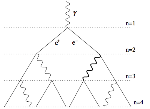
Electromagnetic shower
The Heitler toy model
Electromagnetic shower
Characteristics
- The shower has maximum at $t_{max} = \log(E_0/E_c)/\log2$
- The maximum number of particles is $N_{max} = 2^{t_{max}} = E_0/E_c$
- The shower maximum will be at a depth $X_{max}$: $$X_{max}=X_0 \frac{\log(E_0/E_c)}{\log2}$$
Actual showers also spread laterally mostly due to Coulomb scattering. The lateral spread is a few times the so-called **Moliere unit** equal to $21/E_c$ (MeV).
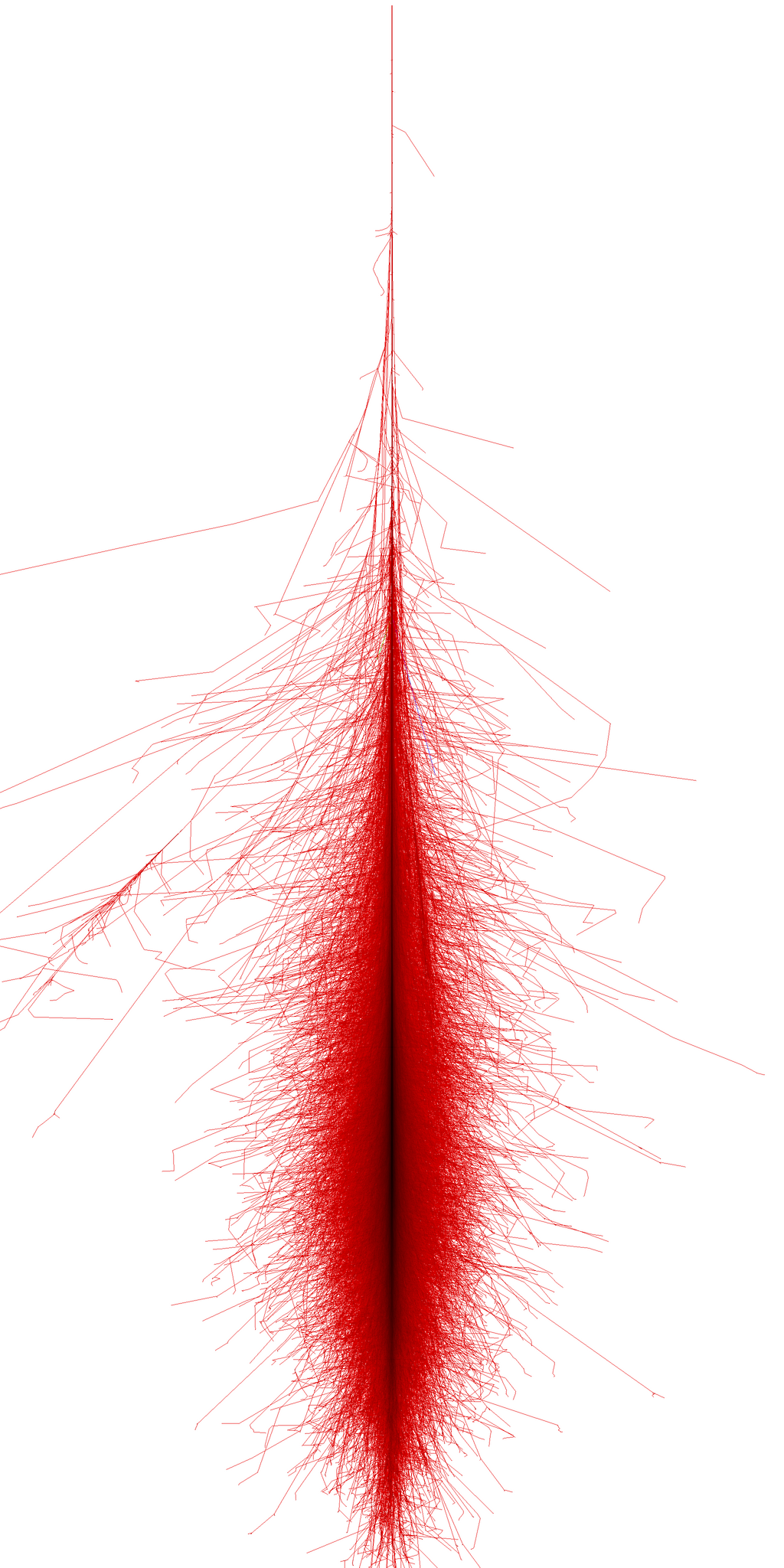
Extensive Air Shower
If instead of an electron a proton initiates the cascade, a nuclear cascade will develope:
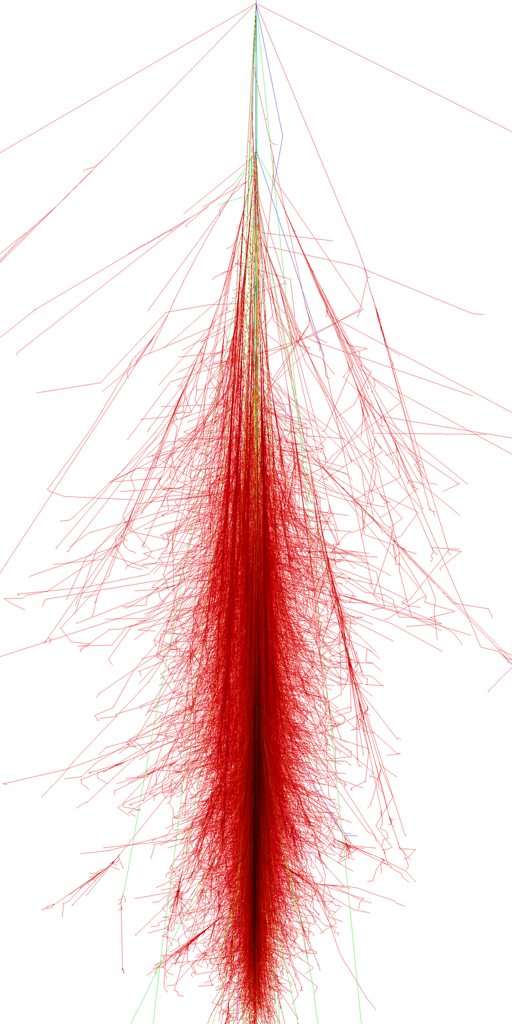
- *Superposition principle*. A nucleus of mass A and energy $E_0$ essentially generates $A$ subshowers of energy $E_0/A$: $$X^{A}_{max} = X_{max}^{p} - \lambda\log A$$ ie, the shower max depends on the mass of the CR primary. In general showers max out deeper in the atmosphere due to longer hadronic interaction length $X_{had} \sim 90 {\rm g/cm}^2$
- Hadronic showers are typically muon-rich with both penetrating muon component and soft EM component reaching ground level.
- Lateral development is much broader than EM cascades with sizes reaching km for UHECR primaries.
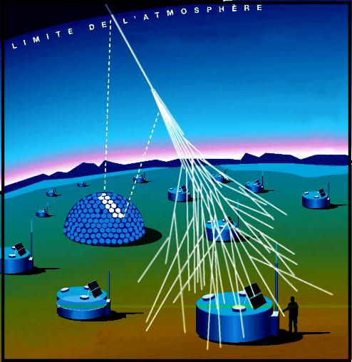
Detection of extensive air showers
Cherenkov Radiation

so the threshold for production is $\beta > \frac{1}{n}$. Most of the components in the air shower will produced abundant Cherenkov light.
Lateral Shower Profile
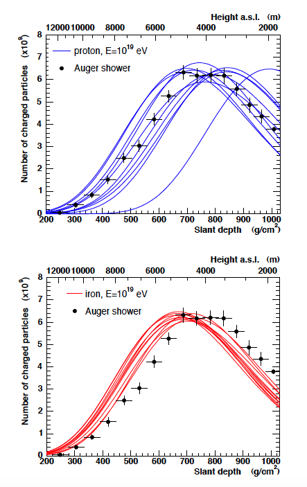
- The CR composition above the knee must be measured by the energy dependence of the position of the shower maximum $X_{max}$. These estimates are subject to large theoretical errors due to lack of knowledge of cross-section behaviors in the extreme forward region.
- Here you can see different realizations of a shower due to an iron or proton primary compared to the same latera distribution of EAS measured in Auger
High Energy Composition

- Composition of the high energy CR spectrum involves only two archetypes: light nuclei (protons) and heavy nuclei (iron).
- The panels at left show Auger / HiRes measurements near GZK cutoff, all favoring at least a mixed composition tending toward heavy at the higher energies.
Sources of Extra Galactic Cosmic Rays
As we shaw, CR in supernova remmants or blast waves can only accelerate CR up to 100 Z TeV. In order to explain CR beyond this energy, one has to invoke other processes such as Non-Linear Diffusion Acceleration, or extremely high magnetic fields (as suggested in Hillas plot).
Binary systems in which a compact object (black hole, neutrino star, pulsar) is permanentely dragging material for an accompaying object (normal star or galaxy) and whirled into an accreation disk can generate enourmouse plasma motions with very strong electromagnetic fields.
 Artistic representation of 4U 0614+091, a X-ray binary. Credit: ESA
Release of gravitational potential energy.
The energy gain of infailling protons corresponds to a variation in the gravitational potential:
$$\Delta E = -\int^{R}_\infty G\frac{m_p M}{r^2} = G\frac{m_p M}{R} $$where $M, R$ are the mass and radius of the central compact object:
For a neutron star ($M\approx 2\times10^{30}$ kg, $R= 10$ km): $\frac{\Delta E}{m_p} \sim 1.32\times 10^{20} {\rm\; erg/g}$
For a black hole ($M\approx 10^8 M_\odot$, $R = R_S = 2\frac{GM}{c^2}$): $\frac{\Delta E}{m_p} \sim 5 \times 10^{20} {\rm\; erg/g}$
How this energy is used to accelerate particles is not clear. There are several models for instance is the Disk dynamo.
Disk dynamo
The idea is that accreatting matter will interact with the magnetic fields of the neutron or black hole. If we equal the variation of gravitational potential to the kinetic energy of the accretting matter we have in the classical approach:
$$\frac{1}{2}m v^2 = \Delta E = G\frac{m M}{R} \rightarrow v =\sqrt{\frac{2 GM}{R}}$$The variable magnetic field of the neutrino star are perpendicular to the direction of the accreation disk generating a Lorentz force:
$$\vec{F} = e (\vec{v} \times \vec{B}) = e\vec{E}$$So the energy obtained is
$$E=\int \vec{F}d\vec{s} = e v B\Delta s$$where $\Delta s$ is the distance over which the force acts. Under plausible assumptions ($v \sim c$, $B= 10^6$ T, $\Delta s = 10^5$ m) energies of $3\times 10^{19}$ eV are possible.
Sources of Extra Galactic Cosmic Rays
The two main candidates for ExtraGalactic Cosmic Rays are:
- Active Galactic Nuclei (AGN)
- Gamma Ray Bursts
Active Galactic Nuclei (AGNs)
Discovered in 1932 by K. Jansky looking for noise in transatlantic radio transmission for the Bell Telephone Labs. He found a persistent noise in the radio from the centre of the Galaxy too loud to be due to thermal black body radiation.
1953 Ginzburg & Shklovski suggested it was due to synchrotron radiation from highly relativistic electrons, confirmed with discovery of predicted polarization in M87 light.
Sandange labeled 3C48 a quasar or quasi-stellar object (it appeared pointlike).
In 1962 3C273 radio source position was found with precision of 1 arcsec, which allowed to find the optical counterpart at z = 0.158 (not 1 star but a galaxy).
In 1963 Hoyle and Fowler speculated that the tremendous emitted energy is due to the gravitational collapse of a very massive object.
AGN Classification
- There is two broad classes: Radio quiet (90%) and Radio Loud (10%) depending on the pressence of jets or not.
- The unified model of ANGs suggests that different AGNs are infact the same object seen from different angles.

Gamma-Ray Burts
- GRBs are short bursts lasting a few seconds of $\gamma$-ray photons from 0.1 - 1 MeV.
- They were discovered in the 60s by the U.S. Vela satellites, which were built to detect gamma radiation pulses emitted by nuclear weapons tested in space as the US suspected the URSS might carry on secret nuclear tests depiste the Nuclear Test Ban Treaty.
They have been hypothesed (given their occurence) to have caused mass extintions events (thousand times since life begun), in particular they are associated with the Ordovician–Silurian extinction.
There is some observational evidence suggesting that progenitor of a GRB are stars undergoing a catastrophic energy release by the end of their lifes $\rightarrow$ Hypernovas
Gamma-Ray Bursts
Sources of UHECR
The accepted phenomenological picuted of GRBs is of a expanding relativistic wind fireball dissipating kinetic energy. The observed afterglow on some GRBs result from the collision of the expanding fireball and the surroundings.
In the fireball, the observed radition is produced by synchrotron emission of shock accelerated electrons, similar to SNRs. Hence, it is likely that protons will be also shock accelerated.
The two conditition for GRBs sources of UHECR are:
The proton acceleration time must be smaller that the wind expansion time (burst duration).
The proton synchrotron loss time must exceed the acceleration time.
These two conditions lead to a constrain in the Lorentz boost factor for GRBs:
$$\gamma \geq 130\left(\frac{E}{10^{20}{\rm\; eV}}\right)^{3/4}\left(\frac{0.01{\rm\; s}}{\Delta t}\right)^{1/4}$$which matches what we see from GRBs. However IceCube has not seen any neutrino associated with GRBs which puts in tension the idea that GRBs can be the only sources of UHECR.
Cosmic Ray Experiments and Detectors
Detection ranges
| Energy Range | Nomenclature | Detection Technique |
|---|---|---|
| 10 MeV - 30 GeV | high (HE) | satellite/space based detector |
| 30 GeV - 30 TeV | very high (VHE) | ground based atmospheric Cherenkov detectors |
| 30 TeV above | ultra high (UHE) and extremely high (EHE) | ground based air-shower and fluorescence detectors. |
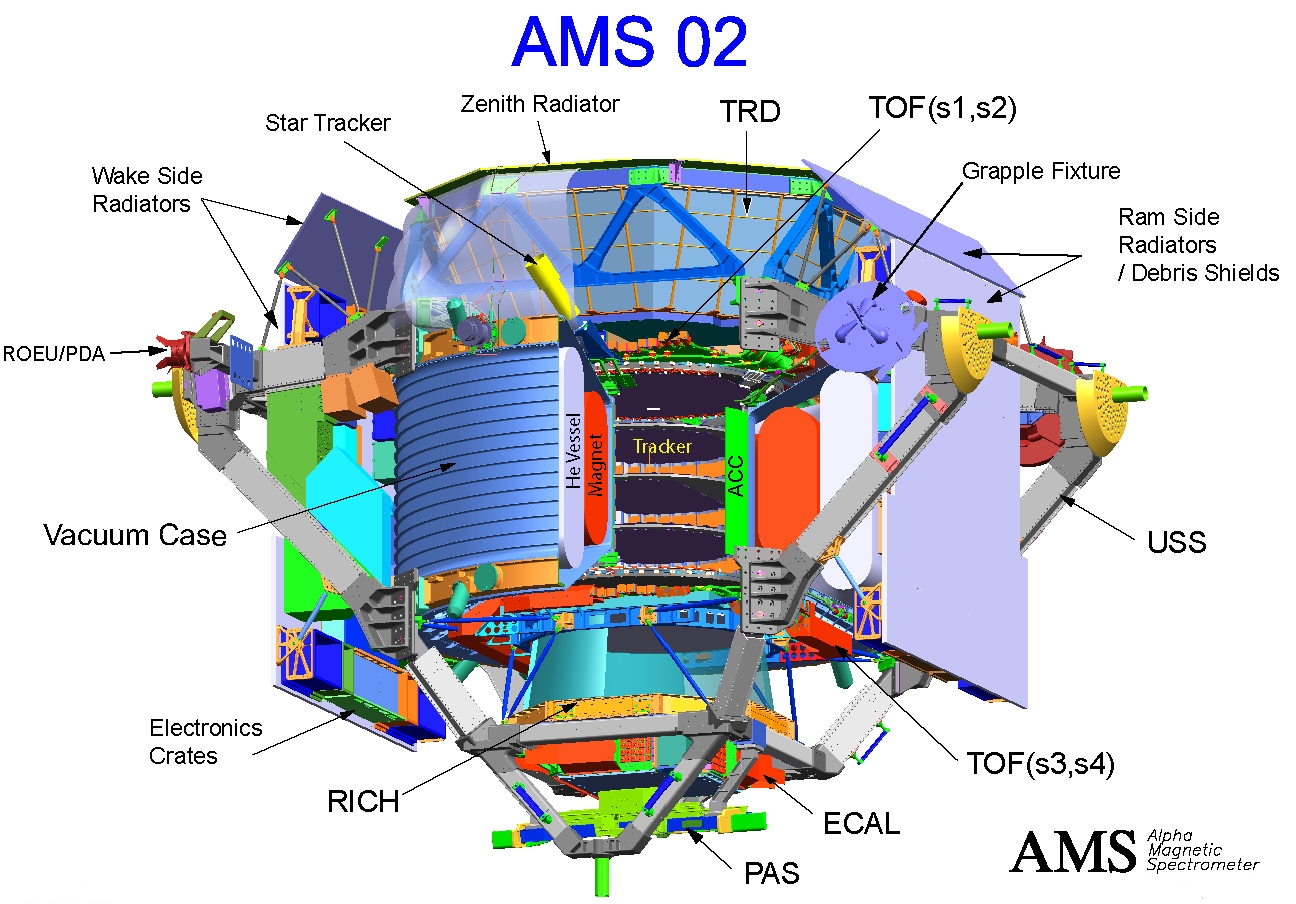
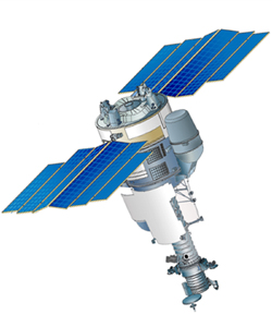
AMS
- Transition radiation detector (TRD): transition radiation is produced when ultra-relativistic charged particle travel through dielectric boundary - emit X-rays which can be used to measure directly $\gamma$ (lorentz factor).
- TOF - time-of-flight system
- Silicon tracking magnetic spectrometer.
- Ring-imaging Cherenkov counter: particle ID in GeV region.
- Electromagnetic calorimeter (ECAL).
PAMELA
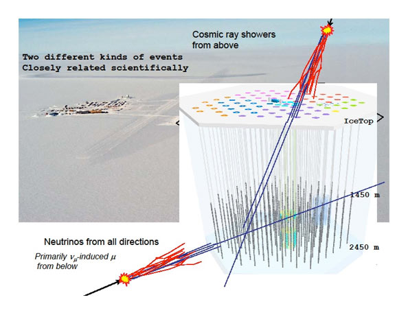
IceTop
IceTop is an array of 81 stations spanning a square kilometer of the Antarctic ice sheet. Each station is located on top of one of IceCube’s strings and holds two tanks of frozen water, each tank equipped with two IceCube sensors or DOMs. It can measure the CR spectrum from $10^{6}$ to 10$^{9}$ GeV.
PIERRE AUGER OBSERVATORY
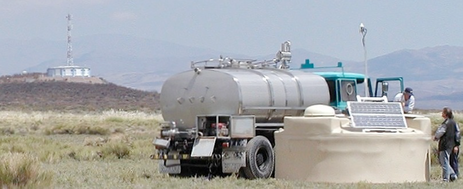
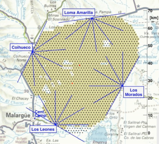
PIERRE AUGER OBSERVATORY
Surface Detector
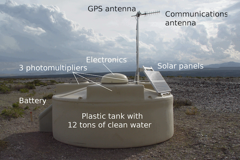
- Each surface detector is 10 m$^2$ plastic tank filled with water. I As the charged particles pass through the water, they emit Cherenkov light which is picked up in 3 down-facing PMTs. 1 VEM (vertical equivalent muon - the standard calibration unit for surface detectors) is approx 100 p.e. in the 3 tubes.
- The distance from tank-to-tank is large - 1.5 km.
- The array is networked to a central facility using radio uplinks and each tank is solar powered.
PIERRE AUGER OBSERVATORY
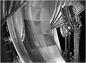
Fluorescence Detector
- 4 FDs - each 12m$^2$ reflector telescopes with 400-pixel PMT camera in the focal plane
- Each camera views about 30$^{\circ} \times $ 30$^{\circ}$ patch of sky
- FD can record shower profiles versus depth and has very good energy resolution from measurement of the fluoresence output of EAS.
- Duty cycle of FD is poor - must be moonless clear night.
What else?
We did not cover:
- Solar modulation of Cosmic Rays and the effect of Earth magnetic fields.
- Cosmic Ray anisotropy in the low and high energies (Compton-Getting effect, etc.)
- The PAMELA and AMS-2 disagreement in the proton and He spectrum.
These could be topics for a research work.
And a paper that contradicts what I explained: Beyond the myth of the supernova-remnant origin of cosmic rays