
Natural Units
It is very common to see use of soi-disant natural units in HEP and HEP-Astro where $\hbar = c = 1$. The correspondence between natural units and physical units can be established by use of
$$\hbar = 6.58 \times 10^{-16} {\;\rm{GeV}\cdot \rm{ns}} = 1\;\Rightarrow 1\;\rm{GeV} = 1.52 \times 10^{15}\;{\rm{ns}^{-1}}$$and
$$c = 30.0\;\rm{cm/ns} = 1 \Rightarrow 30\;\rm{cm} = 1\;\rm{ns}$$In these units there is then only one fundamental dimension:
- Energy and momentum, usually expressed in GeV
- Time and space are GeV$^{-1}$
In Heaviside-Lorentz convention $$\epsilon_0 = \mu_0 = Z_0 = 1$$
$$\alpha = \frac{e^2}{4\pi\epsilon\hbar c} \approx \frac{1}{137} \rightarrow e = \sqrt{4\pi\alpha} \approx 0.303$$import astropy.units as u
from astropy import constants as const
M_Earth = 5.97E24 * u.kg
M_Sun = 1.99E30 * u.kg
M_MW = 1E12 * M_Sun
#By adding the quantity u.kg you can print directly the mass in Kg
print "Mass Earth is: %s" %M_Earth
Sizes, note that the Earth is not a perfect sphere but it will not matter here. 1 A.U. is the mean distance between the Earth and the Sun
R_Earth = 6.371E6 * u.m # meters
R_Sun = 6.955E8 * u.m # meters
AU = 1.496E11 * u.m # meters
Calculate the mean density of Earth and Sun
vol_sphere = lambda r: 4*pi/3*r**3
rho_Sun = M_Sun / vol_sphere(R_Sun)
rho_Earth = M_Earth / vol_sphere(R_Earth)

#Units are preserved along calculations, a unit can be changed calling the .to(u.unit) method
print "Density of Earth:", rho_Earth.to(u.g/u.cm**3)
print "Density of Sun:", rho_Sun
Some definitions (cont.)
Light year:
ly = 1 * u.lyr

print "Number of seconds for light to travel from Sun to Earth:", 1./const.c.to(u.AU/u.s)
print "Meters in a light year:", ly.to(u.m)
The Galaxy (CAPS = Milky Way, no caps = any old galaxy) is roughly a disk 50 kpc in diameter and 500 pc thick
V_Gal =  pi * (25000*u.pc)**2 * 500*u.pc

print "Volume of the Milky Way is approximately: %s " % V_Gal.to(u.m**3)
M_Gal = 1E12 * M_Sun
rho_Gal = M_Gal / V_Gal
print "Average density of Milky Way is %s" % rho_Gal.to(u.g/u.cm**3)
Some Geography
Milky Way
The Sun is 7.6-8.7 kpc from the Galactic Center where there appears to be a supermassive black hole of 1 million solar masses ($M_{\odot} = 1.99\times 10^{30} {\rm kg}$) which coincides with a radio source known as Sagittarius A* .

However the Milky Way is not considered an Active Galactic Nuclei due to the low mass of the black hole. If considered a cylinder it will have a radius of 30 kpc and thickness of 300 pc. Its mass is estimated to be $5.8 \times 10^{11} M_{\odot}$.
Some Geography
Local Group
The Milky Way is surrounded by 54 known satellite galaxies (most of them dwarf galaxies) in a group known as the Local Group. (A dwarf galaxy has $\sim$ billion stars compared to our Milky Ways 200-400 billion stars)
The most notably the Large Magellanic Cloud (50 kpc) and the Small Magellanic Cloud (60 kpc). The LMC mass is $10^{10} M_{\odot}$. Next nearest full-fledged galaxy is Andromeda or M31 ($1.5\times 10^{12} M_{\odot}$) at a distance of approximately 780 kpc. The group contains also other galaxies MW, M31, M33 (Triangulum Galaxy) and it has volume of diameter of about 3 Mpc.

Time
There are several time standards or ways to specify time. A time standard can affect the rate (ie, how long is a day) or reference or point in time, or both. Some standards are:
Mean solar time There are two solar times, the aparent one (also called true one) which depends on latitude and the year and the Mean solar time which the time of mean sun, the difference between the two is called the equation of time. The length of the mean solar day is slowly increasing due to the tidal acceleration of the Moon by the Earth and the corresponding slowing of Earth's rotation by the Moon.
Universal Time (UT0, UT1) Is a time scale based on the mean solar day, defined to be as uniform as possible despite variations in Earth's rotation
International Atomic Time Is the primary international time standard from which other time standards, including UTC, are calculated. TAI is kept by the BIPM (International Bureau of Weights and Measures), and is based on the combined input of many atomic clocks around the world.
Coordinated Universal Time (UTC) is an atomic time scale designed to approximate Universal Time. UTC differs from TAI by an integral number of seconds. UTC is kept within 0.9 second of UT1 by the introduction of one-second steps to UTC. The difference with UT1 is known as DUT1.
Time
JD and MJD
These are not technically standards (or scales), they are just reprentations (formats) of the aforementioned standards typically used in Astronomy:
Julian Date Is the count of days elapsed since Greenwich mean noon on 1 January 4713 B.C., Julian proleptic calendar. Note that this day count conforms with the astronomical convention starting the day at noon, in contrast with the civil practice where the day starts with midnight (in popular use the belief is widespread that the day ends with midnight, but this is not the proper scientific use).
Modified Julian Date Is defined as MJD = JD - 2400000.5. The half day is subtracted so that the day starts at midnight in conformance with civil time reckoning. There is a good reason for this modification and it has to do with how much precision one can represent in a double (IEEE 754) variable. Julian dates can be expressed in UT, TAI, TDT, etc. and so for precise applications the timescale should be specified, e.g. MJD 49135.3824 TAI.
Time
In experiments
Practically speaking, in experiments time comes from one or more of the following sources:
- Atomic clocks (Cs, Rb) -They use the microwave signal that electrons in atoms emit when they change energy levels. These have very good short term performance but a Rb clock left by itself will wander by several ns per day. Cs clocks are perhaps better by a factor of 100x.
- GPS - The GPS gives precision timing too. The system consists of the space segment of O(30) satellites each equipped with Caesium atomic clocks and each constantly getting corrections from the central control facility. GPS broadcasts navigation and time messages synchronized to this ultraprecise time from which the user segment can extract time and space coordinates accurate to O(10) ns and meters, respectively. GPS time is based on the 86400 second day. It indirectly accounts for leap years. There are no leap seconds in GPS time.
Astropy
Time converstions and coordinate conversions are best left to well-tested libraries. SLALIB is a famous set of Fortran libraries that do several transformation. For python I will use Astropy. The Astropy Project is a community effort to develop a single core package for Astronomy in Python and foster interoperability between Python astronomy packages. Is included by default in the Anaconda distribution.
from astropy.time import Time
import datetime
i = datetime.datetime.now()

print ("Today date and time in ISO format: %s" % i.isoformat() )

times = ['1999-01-01T00:00:00.123456789', i.isoformat()]

t = Time(times, format='isot', scale='utc')

print "Todays julian date (UTC) is %.2f" %(t[1].jd)
print "Today's modified julian date (UTC) is %.2f"  %t[1].mjd

dt = t[1] - t[0]

print "The time difference in mjd is %.2f " %dt.value
print "The time difference in seconds is %.2f" %dt.sec
Coordinate Systems
Local coordinates
Coordinate systems are used to map objects position in the sky. They can divided into to:
- Local coordinates system. For example the horizontal coordinate system that uses the observer's local position as reference. It is expressed in terms of altitude (or elevation or zenith) angle and azimuth. Celestials objects change coordinates with time.
Coordinate Systems
Celestial coordinate systems.
Equatorial coordinates: It's defined by an origin at the center of the Earth, a fundamental plane consisting of the projection of the Earth's equator onto the celestial sphere. Coordinates are give by right ascension and declination.
 By Tfr000 (talk) 20:50, 17 April 2012 (UTC) [CC BY-SA 3.0](http://creativecommons.org/licenses/by-sa/3.0) or [GFDL](http://www.gnu.org/copyleft/fdl.html), via Wikimedia Commons
Galactic coordinates: The galactic longitude, $\ell$ is the angular distance Eastward (counterclockwise looking down on the Galaxy from the GNP) from the Galactic Center and the galactic latitude, $b$, is the angular distance outside of the plane of the Galaxy, positive up, negative down. Note that having a large galactic latitude is neither a necessary nor a sufficient condition for an object being extragalactic. This is how to get the image of the Galactic plane on the celestial sphere.
#We call random.multivariate_normal to generate randon normal points at 0
import numpy as np

#For nicer plots (not needed)
import seaborn; seaborn.set()

disk = np.random.multivariate_normal(mean=[0,0], cov=np.diag([1,0.001]), size=5000)
#disk is a list of pairs [l, b] in radians
print disk

figure(figsize=(10,8))
ax = subplot(111, projection='aitoff')
ax.set_title("Galactic Plane in Galactic Coordinates")
grid(True)

ll = disk[:,0]
bb = disk[:,1]

ax.plot(ll, bb, 'o', markersize=2, alpha=0.3)

from astropy import units as u
from astropy.coordinates import SkyCoord

c_gal = SkyCoord(l=ll*u.radian, b=bb*u.radian, frame='galactic')
c_gal_icrs = c_gal.icrs
Because matplotlib needs the coordinates in radians and between −π and π, not 0 and 2π, we have to convert them.
ra_rad = c_gal_icrs.ra.wrap_at(180 * u.deg).radian
dec_rad = c_gal_icrs.dec.radian

figure(figsize=(10,10))
ax = subplot(111, projection="mollweide")
ax.set_title("Galactic plane in equatorial coordinates")
grid(True)
ax.plot(ra_rad, dec_rad, 'o', markersize=2, alpha=0.3)
#NOTE: Normally right ascension is plotted from right (0 deg.) to left (360 deg.)

Special Relativity
Why is it important?
$$\gamma = \sqrt{\frac{1}{1-\beta^2}}\;, \beta = \frac{v}{c}$$- Jets emitted by supermassive black holes have: $\gamma \approx 30 \rightarrow \beta = 0.9984$
- Electrons spiraling in B-field lines of pulsars have: $\gamma \sim 10^7$
- Lorentz factors of protons of $10^{20}$ eV: $\gamma = \frac{E}{m^0_p c^2} = \frac{10^{20}}{1\times 10^9} = 10^{11}$
Two principles:
The Principle of Relativity – The laws by which the states of physical systems undergo change are not affected, whether these changes of state be referred to the one or the other of two systems in uniform translatory motion relative to each other
The Principle of Invariant Light Speed– "... light is always propagated in empty space with a definite velocity [speed] c which is independent of the state of motion of the emitting body."
Lorentz Transformations
As a simple case, consider a reference frame O and and observer in another frame O' moving at constant speed $\beta$ along the $x$ axis:

A Lorentz transformation or boost is the transformation from one inertial reference frame to another. In general it is a $(4\times4)$ matrix which encapsulates the system of equations describing the transformation (in natural units).
$$\begin{align*} t' &= \gamma(t - \beta x) \\ x' &= \gamma(x - \beta t) \\ y' &= y \\ z' &= z \end{align*}$$Lorentz transformation
The matrix form of this transformation is
$$x'^\mu = {\Lambda^\mu}_\nu x^\nu, \; {\Lambda^\mu}_\nu = \begin{pmatrix} \gamma & -\beta\gamma & 0 & 0 \\ -\beta\gamma & \gamma & 0 & 0 \\ 0 & 0 & 1 & 0 \\ 0 & 0 & 0 & 1 \end{pmatrix}$$This is just a particular case of a Lorentz transformation (there is nothing special on the x-axis) and a variable invariant under a Lorentz transformation is called Lorentz invariant or scalar.
The line element $\Delta s^2$ is a Lorentz invariant:
$$\Delta s^2 = \Delta t^2 - \Delta x^2 - \Delta y^2 -\Delta z^2 $$This can be rewritten as the inner product of a 4-vector $x^{\mu}$:
$$\Delta s^2 = x^2 \equiv x^\mu x_\mu = g_{\mu\nu} x^\mu x^\nu$$where metric tensor $g_{\mu\nu}$ is:
$$g_{00} = + 1, g_{11} = g_{22} = g_{33} = - 1 , g_{\mu\nu} = 0, \;\rm{for}\; \mu \neq\nu$$is called the Minkowski space
Consequences of Lorentz transformations
- Relativity of simultaneity. $\Delta t' = 0$ in $O'$ doesn't imply $\Delta t = 0$ in $O$:
- Time dilatation. If $\Delta x = 0$ i.e. the ticks of one clock:
Length contraction. For events satisfying $\Delta t' = 0$:
$$\Delta x' = \frac{\Delta x}{\gamma}$$
Equivalence of mass and energy.
- ...
Equivalence mass and energy
from IPython.display import YouTubeVideo
# Video credit: Minute Physics
YouTubeVideo('hW7DW9NIO9M')
Relativistic kinematics
Four-vectors
We saw that position vectors in Minkowski space become 4-vectors with zeroth component. $x^0 = t$, identified with time. Likewise momentum 4-vector has $p^0 = E$:
$$p= (E, \vec{p})$$$$x= (t, \vec{x})$$We saw that the inner product in Minkowski space is invariant under Lorentz transformations. In this case, the Lorentz invariant is:
$$ s = p_\mu p^{\mu} = m_0^2 = E^2 -{\vec p\cdot \vec p} \rightarrow E^2 = {\vec p\cdot \vec p} +m_0^2$$which is the relativistic energy-momentum relationship.
$$ E = m = \gamma m_0$$One can derive the expresions for relativistic 3-momentum and kinetic energy:
$$|{\vec p}|= \beta E$$$$E_{kin} \equiv E - m_0 = (\gamma -1) m_0$$Relativistic kinematics
Transformation to the Center-of-Momentum System (CMS)
As a concrete example of how 4-vectors aid real calculations, let's take the classic case of a transformation to the center-of-momentum system (CMS), that is, a coordinate frame where the total three-momentum $\vec p = 0$. In this case the invariant square of a system is equal to the total CMS energy square or:
$$\sqrt{s} = E_{CMS}$$In the case of colliding particles, A and B, with energies $(E_A)$ and $(E_B)$, and 3-momenta $(\vec{p}_A)$ and $(\vec{p}_B)$:
$$\begin{align} s = p^2 &= (E_A + E_B)^2 - (\vec{p}_A + \vec{p}_B)^2 \\ &= m_A^2 + m_B^2 + 2E_AE_B - 2(\vec{p}_A \cdot \vec{p}_B)\\ &= m_A^2 + m_B^2 + 2E_AE_B( 1 - \beta_A\beta_B\cos \theta)\\ &= E_{cms}^2 \end{align}$$The energy available for new particle creation is $\epsilon = \sqrt{s} - m_B - m_A$. If $E_A \gg m_A$ and $E_B \gg m_B$ then
$$\epsilon^2 \approx 2 (E_A E_B - \vec{p}_A \vec{p}_B )$$
Relativistic kinematics
Fixed-target experiment
If the target particle B is at rest in the laboratory system (as is the case in accelerator fixed-target experiments or UHE cosmic rays striking nucleons in the atmosphere, or ...) then $(E_B = m_B)$ and $(\vec{p}_B = 0)$. In this case,
$$\begin{align} E_{cms}^2 = m_A^2 + m_B^2 + 2E_Am_B \end{align}$$which in the ultra-relativistic limit where energies are much higher than the masses $(E \gg m)$ simplifies to
$$\begin{align} \epsilon = E_{cms} \simeq \sqrt{2m_BE_A} \end{align}$$Equivalently, the threshold energy of the beam particle A needed to produce a particle of mass $(m_*)$ at rest in the boosted frame is $$\begin{align} E{A,\mathrm{thresh}} = \frac{m*^2}{2m_B} \end{align}$$
Relativistic kinematics
- Example 1: $\pi^0$ production. Considering the photoproduction of pion on a target proton at rest mass: $$\gamma + p \rightarrow p + \pi^0$$
4-vector Calculations in CMS
Collider experiment
In the case of a collider experiment where beam particles A and B are counter-circulating in an accelerator and collide head-on, then
$${\vec p}_{A}\cdot{\vec p}_{B} = -|{\vec p}_{A}||{\vec p}_{B}|$$and the equation of the 3-momenta ${\vec p}_A$ becomes
$$\begin{align} s = E_{cms}^2 = m_A^2 + m_B^2 + 2(E_AE_B + |{\vec p}_{A}||{\vec p}_{B}|) \rightarrow \epsilon^2 \simeq 4E_AE_B \end{align}$$in the relativistic limit where mass can be ignored. This in turn has the consequence that in a collider experiment the energy available in the CMS to produce new particles rises linearly with beam energy when $E_A = E_B$.
Nevertheless, it is still the case that the CMS energies probed by astroparticles exceeds the LHC's reach by a factor of 10: consider an UHECR proton at $E_A = 10^{10}\;\rm{GeV}$ interacting with a proton ($m_B = 1 \rm{GeV}$) at rest in the atmosphere.
m_A = m_B = 1. #GeV
E_A = 1e10 #GeV
E_cms = sqrt(m_A*m_A + m_B*m_B + 2*(E_A*m_B))/1.e3
print 'E_cms = %.1f TeV' % E_cms
Two-body decay in CMS
The CMS is also useful to estimate the energy of two particles from the decay of a particle with mass $M$. If a particle A decays into 1 $m_1$ and 2, $m_2$, we have that in the CMS the particle A has ${\vec p_A} = {\vec p_{CMS}} = 0$. Then the invariant is given by: $$ s = M^2 = (E_1 + E_2)^2 - (\vec{p}_1 + \vec{p}_2)^2 $$ where ${\vec p_1} = -{\vec p_2}$. It can be proved that the energies in the CMS are given by:
$$E_1 = \frac{1}{2M}(M^2 + m_1^2 - m_2^2)$$$$E_2 = \frac{1}{2M}(M^2 + m_2^2 - m_1^2)$$and the momentum:
$${|\vec p_1|^2} = E_1^2 - m_1^2 = \frac{1}{4M^2}(M^4 - 2M^2(m_1^2 + m_2^2) + (m_1^2 + m_2^2)^2) = {|\vec p_2|^2}$$Energies and momentums are fixed, the only unknowns are the angles.
Cosmology
Red-shift
Red-shift is the shift (towards red) in the electromagnetic spectrum and is defined as:
| $$\begin{equation} z=\frac{\lambda_{obs} - \lambda_{emit}}{\lambda_{emit}} \end{equation}$$ |

|
If a source of the light is moving away from an observer, then redshift (z > 0) occurs; if the source moves towards the observer, then blueshift (z < 0) occurs. This is true for all electromagnetic waves and is explained by the Doppler effect. Consequently, this type of redshift is called the Doppler redshift.
Relativistic Redshift
The wavefront moves with velocity $c$, but at the same time the source moves away with velocity $v$, so $\lambda+v t=ct$. The period in the reference system of the source is given by:
$$t_s = \frac{\lambda}{c-v} = \frac{c}{(c-v)f_s} = \frac{1}{(1-\beta)f_s},$$Remember that when a reference $O_s$ was moving at speed $\beta$ from a another reference $O_{obs}$, the time relatiom was:
$$\Delta t = \gamma(\Delta t_{obs} - \beta \Delta x_{obs})$$Since $\Delta x_{obs} =0$ (we are just measuring when the crest of the waves arrive), then the time observed $t_{obs}$ in the reference system O is given:
$$t_o = \frac{t}{\gamma}$$,
The corresponding observed frequency is $$f_o = \frac{1}{t_o} = \gamma (1-\beta) f_s = \sqrt{\frac{1-\beta}{1+\beta}}\,f_s$$ The ratio $$\frac{f_s}{f_o} = \sqrt{\frac{1+\beta}{1-\beta}}$$
is called the Doppler factor of the source relative to the observer. The corresponding wavelengths are related by $$\frac{\lambda_o}{\lambda_s} = \frac{f_s}{f_o} = \sqrt{\frac{1+\beta}{1-\beta}}$$ and the resulting redshift
$$z = \frac{\lambda_o - \lambda_s}{\lambda_s} = \frac{f_s - f_o}{f_o}$$can be written as $$z = \sqrt{\frac{1+\beta}{1-\beta}} - 1.$$
In the non-relativistic limit (when $v \ll c$) this redshift can be approximated by $z \simeq \beta = \frac{v}{c}$ corresponding to the classical Doppler effect.
When interpreted as a relativistic Doppler shift from object receeding at velocity $\beta$, this is:
$$\lambda = \sqrt{\frac{1+\beta}{1-\beta}}\lambda_0 \simeq (1+\beta)\lambda_0$$for near, only mildly relativistic $v \ll c$, objects so that the redshift $z$ is approximately equal to the velocity.
Hubble expansion
When ploting their redshift (ie speed) as function of distance (measured with the techniques we saw, parallax, etc.) Hubble found a correlation between redshift and radial distance from Earth:

Note that $H_0$ has only units of time$^{-1}$ we explicitely write the other dimensions to better understand its meaning.
But Doppler redshift does not depends on distance! so there is also a Cosmological redshift. In this case the redshift is not due to relative velocities, the photons instead increase in wavelength and redshift because the spacetime through which they are traveling is expanding.
Hubble expansion
But we said that for midly relativistic objects (and galaxies are moving at midly relativistic speeds) we can approximate $z \approx \beta$ so we can use $z$ to estimate distances!:
$$r \simeq \frac{c}{H_0}z \simeq 4000\;\rm{Mpc}\cdot z$$However is bit tricky, is it the distance when light was emitted or when ligth arrived?
If we assume that the rate of expansion (ie H) is essentially constant (it is not!) the age of the Universe can be estimated to increase by a factor $e$ every $t_{\mathrm{Hubble}} = \frac{1}{H_0} = 14\times 10^9\rm{yr}$ which is the Hubble time.
The common interpretation of the expansion is that we are living in a Universe that can be thought of lying on the surface of a balloon. Distances between objects (points on the ballon) on this manifold are expressed as:
$$r(t) = R(t)r_0$$where $R(t)$ is a scale factor, depending on the time, and $r_0$ is a comoving coordinate without time dependence or current distance if we assume $R(0) = 1$, but sometimes its better to explicitelly use a normalized scale factor as $a(t) = R(t)/R(0)$
Brooklyn is not expanding! Annie Hall
Are we expanding with the Universe?
Cosmological principle
The cosmological principle is the notion that the distribution of matter in the Universe is homogeneous and isotropic when viewed on a large enough scale.
- Homogeneity states that the distribution of matter is even in each epoch.
- Isotropy states that there are no prefered directions in the distribution of matter in space.
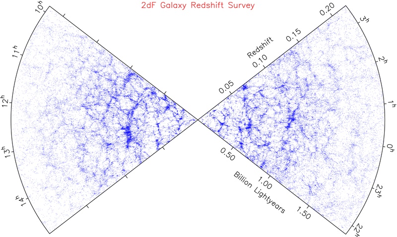
The End of Greatness is an observational scale discovered at roughly 100 Mpc where the lumpiness seen in the large-scale structure of the universe is homogenized and isotropized, this together with the isotropy of the CMB reinforced the idea of the Cosmological Principle.
However, in 2013 a new structure 3 Gpc wide has been discovered, the Hercules–Corona Borealis Great Wall, which puts doubt on the validity of the cosmological principle...
Friedmann–Lemaître-Robertson-Walker
So we are looking for a Universe that is isotropic, homogeneous and it is expanding. The metric that describes such a Universe is given by the Friedmann–Lemaître-Robertson-Walker metric:
$$ds^2 = dt^2 - R(t)^2 d \Sigma(k)^2 = dt^2 - a^2(t)R^2_0\left[\frac{dr^2}{1 - kr^2} + r^2(d\theta^2 + sin^2\theta d\phi^2)\right]$$where $d\Sigma(k)$ refers to the spatial 3-dimentional metric depending on the curvature parameter $k$ which takes the values +1, 0, -1, and we used the normalized form of the scale factor $a(t) = R(t)/R_0$.

The evolution of the scale parameter as in the case of wavelength (to be proved):
$$a(t) = \frac{1}{1+z}$$Friedman equations
Einstein's oringanl field equations are:
$$R_{\mu\nu} - \frac{1}{2}Rg_{\mu\nu} = 8 \pi GT_{\mu\nu}$$In Newtonian gravity, the source is mass. In special relativity, is a more general concept called the energy-momemtum tensor, which may be modeled as a perfect fluid:
$$T_{\mu\nu} = (\rho + p)U_\mu U_\nu + pg_{\mu\nu}$$were $U_\mu$ is the fluid four-velocity. The FLRW metric solution to the Einstein equations can be reduced to the two Friedmann equations:
$$H^2 \equiv \left(\frac{\dot a}{a}\right)^{2} = \frac{8\pi G}{3}\rho - \frac{kc^{2}}{a^2R^2_0} $$and
$$\frac{\ddot a}{a} = -\frac{4\pi G}{3}(\rho + 3p)$$The cosmological constant
Einstein was interested in finding $\dot{a} = 0$ (ie static) solutions. This can be achieved if $k= + 1$ and $\rho$ is appropriately tuned.But $\ddot a$ will not vanish in this case. Einstein therefore modified his equations to:
$$R_{\mu\nu} - \frac{1}{2}Rg_{\mu\nu} + \Lambda g_{\mu\nu}= 8 \pi GT_{\mu\nu}$$and with this modification the Friedmann equations are:
$$ \begin{align*} H^2 &= \left(\frac{\dot a}{a} \right)^2 = \frac{8\pi G}{3}\rho + \frac{\Lambda}{3} - \frac{kc^{2}}{a^2R^2_0} \\ \frac{\ddot a}{a} &= -\frac{4\pi G}{3}(\rho + 3p) + \frac{\Lambda}{3} \end{align*} $$The discovery by Hubble that the Universe is expanding eliminated the empirical need for a static world. However, we believe that $\Lambda$ is actually nonzero, so Einstein was right after all. Assuming that cosmological constant is due to the vacuum energy, most quantum field theories predict a $\Lambda$ that is 120 orders of magnitude larger than the observational values! this is so-called cosmological constant problem.
Cosmological Constants
For any value of $H$ there is a critical density such as the geometry is flat ($k=0$):
$$\rho_{crit} = \frac{3H^2}{8\pi G}$$It is convenient to measure the the total energy density in terms of critical density by introducing the density parameters:
$$\Omega\equiv\frac{\rho}{\rho_{crit}} = \left(\frac{8\pi G}{3H^2}\right)\rho$$In general the energy density will have contributions of distinct components so whe can defined:
$$\Omega_i\equiv\frac{\rho_o}{\rho_{crit}} = \left(\frac{8\pi G}{3H^2}\right)\rho_i$$where $i$ stands for matter (or dust) and radiation.
For t = 0
$$H_0^2\Omega_0 = \frac{8\pi G}{3}\rho_0$$Evolution of the Cosmological Constants
In general the energy density will have contributions of distinct components which will evolve differently with the Universe expansion:
- Massive particles with negligible velocities are known in cosmology as dust or simply matter. Their density scales as the number density times their rest mass. Their number density scales as the inverse of the volume while the rest mass is constant: $\rho_M \propto a^{-3}$
- Relativistic particles are known as radiation (although it is not only photons) and their energy density is the number density times the particle energy, the latter is proportional to $a^{-1}$ (as they redshift with expansion) and so: $\rho_r \propto a^{-4}$
- Vacuum energy does not change as universe expand so we can define a $\rho_\Lambda \equiv \frac{\Lambda}{8\pi G} \propto a^0$
- It is useful to pretend that $-ka^{-2}R_0^{-2}$ represents an effective curvature energy density defining $\rho_k \equiv -(3k/8\pi G R^2_0)a^{-2}$.
Given this evolution it is possible to write:
$$ H^2(t) = H^2_0 [\Omega_M(1+z)^3 + \Omega_r(1+z)^4 + \Omega_k(1+z)^2 +\Omega_\Lambda]$$Observational results
There are good reasons to believe that the energy density of radiation is much less than matter, as photon contrinute only to $\Omega_r \sim 5 \times 10^{-5}$ mostly in the CMB. Therefore is useful to parametrize the universe today as $\Omega_k = 1 - \Omega_M - \Omega_\Lambda$.
Direct measures of the Hubble constant.. The most reliable result on the Hubble constant comes from the Hubble Space Telecope Key Project. They use the Cepheids to obtain distances to 31 galaxies (They also use Type Ia Supernovae). A recent study with over 600 Cepheids yileded the number $H_0 = 73.8 \pm 2.4 {\rm\;km\;s^{-1}\; Mpc^{-1}}$. The indirect measurement from Planck Collaboration gives somehow a lowe value (this discreptancy as well as the comic distance-ladder method are under investigation).
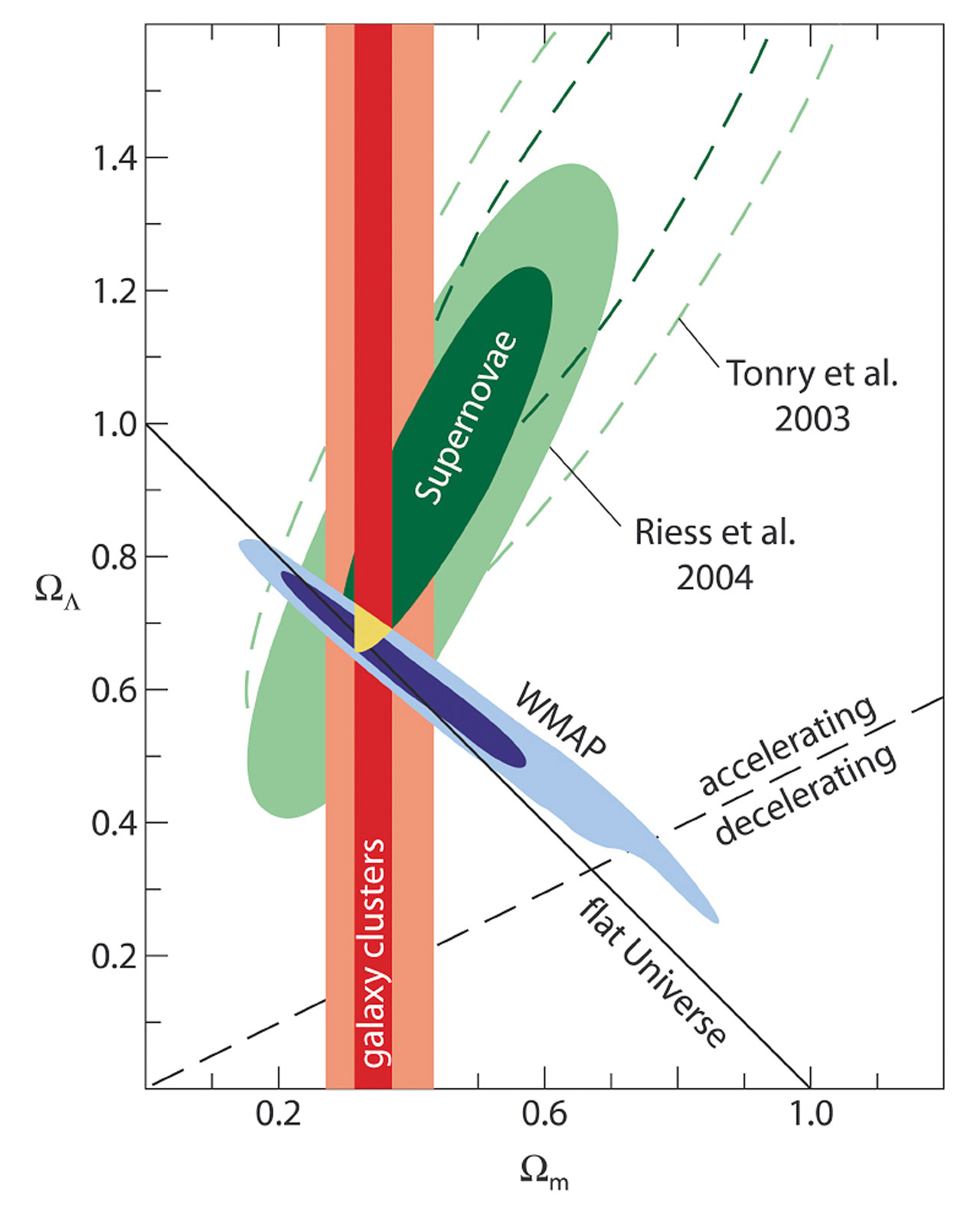
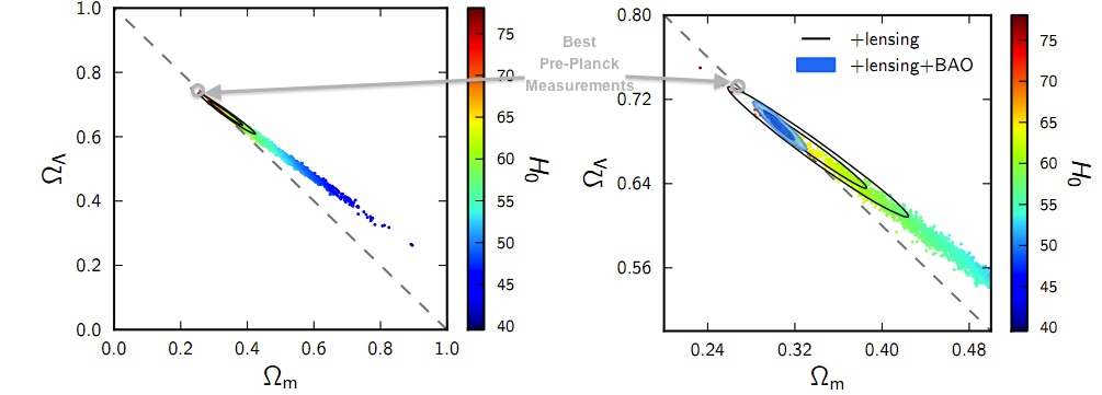
Supernovae. Two major studies, the Supernova Cosmology Project and the High-$z$ Supernova Search Team, found evidence for an accelerating Universe. When combined with the CMB data indicating flatness (ie $\Omega_k = 0 \rightarrow \Omega_M + \Omega_\Lambda = 1$), the best-fit values were $\Omega_M \approx 0.3$ and $\Omega_\Lambda \approx 0.7$)
- Cosmic Microwave Background. See next.
And the amount of anisotropy at the multipole moment $\ell$ via the power spectrum
$$C_\ell = \langle |a_{\ell m}|^2 \rangle$$, $$\theta = \frac{180^{\circ}}{\ell}$$
Observational results
Cosmic Microwave Background
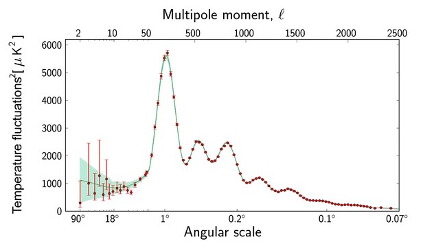
The power spectrum of the CMB represents the anisotropies of the CMB as a function of the angular scale. The typical spectrum features a plateu at large angular scales (small $\ell$) followed by some oscillatory features (aka acoustic peaks or Doppler peak). These peaks represent the oscillation of photon-baryon fuild around the decoupling. The first peak at $\ell \sim 200$ probes the spatial geometry, while the relative heights probe the baryon density. The position of the first peak constrains the spatial geometry in a way consistent with a flat Universe ($\Omega_k \sim 0$)
Age of Universe
We have shown the evolution of the Hubble expansion as a function of the redshift using the clousure parameters. We know that
$$H(z) = \frac{\dot a}{a} = -\left(\frac{{\rm d}z/{\rm d}t}{(1+z)}\right) \rightarrow {\rm d}t = -\frac{{\rm d}z}{(1+z)H(z)}$$Astropy also has some built-in cosmologies using the values extracted from experiments. And so the age of the universe can be calculated as (where $z=0$ corresponds to today $t_0$):
$$\int_{0}^{t_0} {\rm d} t = t_0 = \frac{1}{H_0} \int^\infty_0 \frac{{\rm d}z}{\Omega_M(1+z)^4 + \Omega_r(1+z)^5 + \Omega_k(1+z)^3 +\Omega_\Lambda(1+z)]} $$Assuming a flat Universe $\Omega_k =0$ and ignoring the radiation $\Omega_r \ll \Omega_M$ the integral gets simplified to:
$$H_0 t_0 = \frac{1}{3\sqrt{1 - \Omega_M}}{\rm In}\left(\frac{1+\sqrt{1 - \Omega_M}}{1 - \sqrt{1- \Omega_M}}\right)$$where we used $1 = \Omega_\Lambda + \Omega_M$
def H0T0(omega):
    return 1/(3*np.sqrt(1-omega))*np.log((1 + np.sqrt(1-omega))/(1 - np.sqrt(1-omega)))

omega = np.arange(0, 1.0, 0.01)

ax = subplot(111)
ax.plot(omega, H0T0(omega))
ax.set_xlabel("$\Omega_M$", fontsize=20)
ax.set_ylabel("$H_0 t_0$", fontsize=20)
ax.set_title("Age for a Flat Universe")

print " For Omega_M = 0.7 the value of H0T0 is: %.3f" %H0T0(0.3)

For $\Omega_M = 0.70$ and $\Omega_\Lambda = (1 - \Omega_M) = 0.70$ one finds $H_0 t_0 = 0.964$ so that $t_0 \approx = 0.96/H_0 = 13.5$ Gyr. Larger than the assumption we did with a constant $H_0$.
#Now lets use the cosmology built in astropy
from astropy.cosmology import Planck13, WMAP7
print Planck13.age(0)
print WMAP7.age(0)
#We are going to plot the H "constant" to verify that is not a constant

z = np.arange(0.001, 2, 0.01)
ax = subplot(111)
#Let's assume midly relativistic ie z ~ v: so d = z* c/H
ax.plot(z, z*const.c.to(u.km/u.s).value/Planck13.H(0).value, label="H_0")
ax.plot(z, z*const.c.to(u.km/u.s).value/Planck13.H(z).value, label="H(z)")
legend()
ax.set_xscale("log")
ax.set_yscale("log")
ax.set_xlabel("$z$", fontsize="20")
ax.set_ylabel("D (Mpc)", fontsize="20")
